Sea $ f : \mathbb{R}^3 \rightarrow \mathbb{R}$ sujeta a dos restricciones:

$g_1 (x, y, z) = 0$

$g_2 (x, y, z) = 0$

Hipótesis:

Para todo $ \vec{p} \in {g_1}^{-1} (0) \cap {g_2}^{-1} (0) \neq \emptyset$ los gradientes $\nabla g_1 (\vec{p})$ y $\nabla g_2 (\vec{p})$ son linealmente independientes.

Sea $\vec{q}$ un punto en donde $f\big|_{{g_1}^{-1} (0) \cap {g_2}^{-1} (0)}$ alcanza un valor extremo, le aplicamos el teorema de la función implícita a $G : \mathbb{R}^3 \rightarrow \mathbb{R}^2$ tal que $(x, y, z) \rightarrow \big( g_1 (x, y, z), g_2 (x, y, z) \big)$

Sin pérdida de generalidad, supongamos $\begin{align*} x = h_1 (z) \\ y = h_2 (z) \end{align*}$

$f\big|_{{g_1}^{-1} (0) \cap {g_2}^{-1} (0)}$ puede verse como una función $\mathcal{I} \subseteq \mathbb{R} \rightarrow \mathcal{J} \subseteq \mathbb{R}$ tal que

$z \rightarrow f \big( h_1 (x, y, z) , h_2 (x, y, z) , z \big)$

Entonces $ (x, y, z)$ es solución del sistema de ecuaciones cerca del punto $\vec{q}$ si y sólo si

$x = h_1 (z)$

$y = h_2 (z)$

$\alpha (z) = \big( h_1 (x, y, z) , h_2 (x, y, z) , z \big)$ parametriza un «pedacito» de curva (que pasa por $\vec{q}$).

Maximizar $f ( \alpha (z) )$

Derivando

$\nabla f \big( \alpha (z) \big) \cdot {\alpha \, }’ (z) = \Big( \dfrac{\partial f}{\partial x} , \dfrac{\partial f}{\partial y} , \dfrac{\partial f}{\partial z} \Big) \cdot \Big( {h_1}’ , {h_2}’ , 1 \Big) = 0$

$\dfrac{\partial f}{\partial x} {h_1}’ \, + \, \dfrac{\partial f}{\partial y} {h_2}’ \, + \, \dfrac{\partial f}{\partial z} = 0$

Luego $\nabla f$ es ortogonal a ${\alpha \, }’$, es decir, $\nabla f$ está en el plano generado por $\nabla g_1$ y $\nabla g_2$, es decir,

$$\nabla f = \lambda_1 \nabla g_1 \, + \, \lambda_2 \nabla g_2$$

El teorema de la función implícita se usa para determinar si el conjunto de soluciones de un sistema de ecuaciones es una curva suave o una superficie suave o una variedad suave.

Una ecuación con dos variables

$f (x, y) = 0$

$f^{-1} (0) = \big\{ (x, y) \in \mathbb{R}^2 \big| f (x, y) = 0 \big\}$ conjunto de nivel.

Supongamos que conocemos un punto en $f^{-1}(0)$. Las posibilidades para este conjunto de nivel son:

*) Podría ser un punto,

**) podría ser una o varias curvas que se cruzan, o

***) podría ser una curva con picos.

Para que sea una curva sin picos se debe cumplir las siguientes condiciones:

$f : \mathbb{R}^2 \rightarrow \mathbb{R} $ de clase $\mathcal{C}^1$, $f^{-1} (0) \neq \emptyset$

$\nabla f (p) \neq \vec{0}$, para todo $p \in f^{-1} (0)$

Entonces, $f^{-1} (0)$ es una curva suave sin autointersecciones.

Si $\nabla f (p) \neq \vec{0}$, entonces

a) $\dfrac{\partial f}{\partial x} (p) \neq 0$ entonces existe una función $g$ tal que, cerca de $p$, $f^{-1} (0)$ es la gráfica de $x = g (y)$; o

b) $\dfrac{\partial f}{\partial y} (p) \neq 0$ entonces existe una función $h$ tal que, cerca de $p$, $f^{-1} (0)$ es la gráfica de $y = h (x)$

Una ecuación con tres variables

$f (x, y, z) = 0$

$f^{-1} (0) = \big\{ (x, y, z) \in \mathbb{R}^3 \big| f (x, y) = 0 \big\}$ conjunto de nivel.

Supongamos que conocemos un punto en $f^{-1}(0)$. Las posibilidades para este conjunto de nivel son:

*) Podría ser un punto,

**) podría ser una o varias superficies que se cruzan, o

***) podría ser una superficie con «pellizcos».

Condiciones

$f^{-1} (0) \neq \emptyset$, con $f : \mathbb{R}^3 \rightarrow \mathbb{R}$ de clase $\mathbb{C}^1$

$\nabla f (\vec{p}) \neq \vec{0}$ para todo $\vec{p} \in f^{-1} (0) $

Entonces $f^{-1} (0) $ es una superficie suave sin autointersecciones.

Si $\nabla f (\vec{p}) \neq \vec{0}$ entonces:

i) $\dfrac{\partial f}{\partial x} (\vec{p}) \neq 0$ entonces existe $g $ tal que $ x = g (y, z)$

ii) $\dfrac{\partial f}{\partial y} (\vec{p}) \neq 0$ entonces existe $h $ tal que $ y = h (x, z)$

iii) $\dfrac{\partial f}{\partial z} (\vec{p}) \neq 0$ entonces existe $\varphi $ tal que $ z = \varphi (x , y)$

Dos ecuaciones con tres variables

$f (x, y, z) = 0$

$g (x, y, z) = 0$

Supongamos que el conjunto de soluciones es no vacío.

¿Qué podría ser?

*) Podría ser un punto.

**) Podría ser una o varias curvas que se cruzan.

***) Podría ser una curva con picos.

Condición

Sea $F : \mathbb{R}^3 \rightarrow \mathbb{R}^2$ tal que

$F (x, y, z) = \big( f (x, y, z), g (x, y, z) \big)$

El conjunto de soluciones del sistema de ecuaciones

$f (x, y, z) = 0$

$g (x, y, z) = 0$

podemos verlo de dos formas

a) como la intersección de dos conjuntos de nivel

$$ f^{-1} (0) \cap g^{-1} (0)$$

b) como la imagen inversa de $(0,0)$ bajo $ F $, es decir $ F^{-1} (0, 0).$

${}$

Si pedimos que $\nabla f (\vec{p}) \neq \vec{0} $ y que $\nabla g (\vec{p}) \neq \vec{0} $ para todo $\vec{p} \in f^{-1} (0) \cap g^{-1} (0)$, lo único que podemos concluir es que localmente, el conjunto de soluciones es la intersección de dos superficies suaves

$ \nabla f = ( 0, 0, 1) \; \; \; \; \; \; \; \; \; \; f (x, y, z) = z$

$ \nabla g = ( 2x, \, – \, 2y, \, – \, 1 ) \; \; \; \; \; \; \; \; \; \; g (x, y, z) = x^2 \, – \, y^2 \, – \, z$

$f^{-1} (0) $ plano $z = 0$

$ g^{-1} (0)$ es la silla $ z = x^2 \, – \, y^2$

En el siguiente enlace, puedes observar las gráficas de $f^{-1} (0) $ y $g^{-1} (0) $, así como su intersección.

https://www.geogebra.org/classic/y8cum2au

En este caso la intersección consiste de dos rectas que se cruzan. Para evitar situaciones como esta necesitamos que

$\nabla f (\vec{p})$ y $\nabla g (\vec{p})$ sean linealmente independientes en todo $ \vec{p} \in f^{-1} (0) \cap g^{-1} (0)$.

La matriz de la diferencial de $F$ en $\vec{p}$ es

$$\begin{pmatrix} \dfrac{\partial f}{\partial x} (\vec{p}) & \dfrac{\partial f}{\partial y} (\vec{p}) & \dfrac{\partial f}{\partial z} (\vec{p}) \\ \\ \dfrac{\partial g}{\partial x} (\vec{p}) & \dfrac{\partial g}{\partial y} (\vec{p}) & \dfrac{\partial g}{\partial z} (\vec{p}) \end{pmatrix}$$

¿Qué condiciones debemos pedir en este caso?

Que los gradientes de $f $ y $g$ sean linealmente independientes.

Equivalentemente, que la matriz tenga rango 2.

Equivalentemente, que al menos un subdeterminante de 2×2 (un menor) sea distinto de CERO. De esta última condición, tenemos tres posibilidades:

a) $\begin{vmatrix} \dfrac{\partial f}{\partial x} (\vec{p}) & \dfrac{\partial f}{\partial y} (\vec{p}) \\ \\ \dfrac{\partial g}{\partial x} (\vec{p}) & \dfrac{\partial g}{\partial y} (\vec{p}) \end{vmatrix}\neq 0$

b) $\begin{vmatrix} \dfrac{\partial f}{\partial x} (\vec{p}) & \dfrac{\partial f}{\partial z} (\vec{p}) \\ \\ \dfrac{\partial g}{\partial x} (\vec{p}) & \dfrac{\partial g}{\partial z} (\vec{p}) \end{vmatrix}\neq 0$

c) $\begin{vmatrix} \dfrac{\partial f}{\partial y} (\vec{p}) & \dfrac{\partial f}{\partial z} (\vec{p}) \\ \\ \dfrac{\partial g}{\partial y} (\vec{p}) & \dfrac{\partial g}{\partial z} (\vec{p}) \end{vmatrix}\neq 0$

Si a) se cumple, entonces

$x = h_1 (z)$

$y = h_2 (z)$

Si b) se cumple, entonces

$x = g_1 (y)$

$z = g_2 (y)$

Si c) se cumple, entonces

$y = \varphi_1 (x)$

$z = \varphi_2 (x)$

Veamos un ejemplo de este tipo.

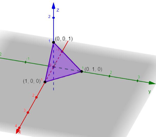
Sea $F (x, y, z) = \big( x^2 + y^2 + z^2 \, – \, 1 , x + y + z \, – \, 1\big)$

$ f (x, y, z) = x^2 + y^2 + z^2 \, – \, 1 = 0$, esfera de radio 1 y centro $(0, 0, 0)$, y

$ g (x, y, z) = x + y + z \, – \, 1 = 0$, plano que pasa por: $(1, 0, 0)$, $(0, 1, 0)$ y $(0, 0, 1)$.

En la siguiente animación puedes observar las gráficas de $f$ y $g$.

https://www.geogebra.org/classic/yvduga9b

La matriz de la diferencial de $F$ en $\vec{p}$ es

$\begin{pmatrix} 2x & 2y & 2z \\ \\ 1 & 1 & 1 \end{pmatrix}$

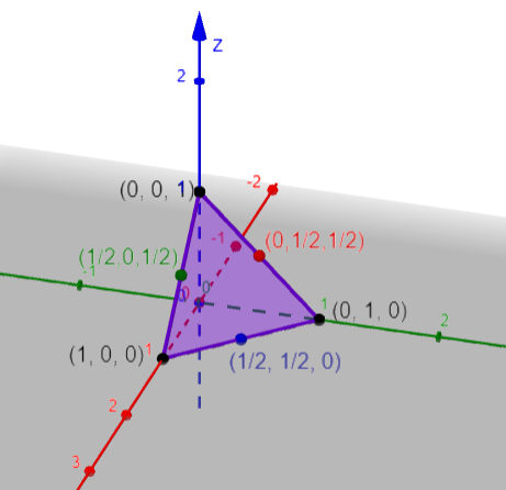
Tomemos el punto $( 0, 0 , 1)$, luego analizamos los menores en ese punto:

$\begin{vmatrix} 0 & 0 \\ \\ 1 & 1 \end{vmatrix} = 0$

$\begin{vmatrix} 0 & 2 \\ \\ 1 & 1 \end{vmatrix} = – \, 2 \neq 0 $ entonces $x = g_1 (y) ; z = g_2 (y)$

$\begin{vmatrix} 0 & 2 \\ \\ 1 & 1 \end{vmatrix} = – \, 2 \neq 0 $ entonces $y = \varphi_1 (x) ; z = \varphi_2 (x)$

Luego, puedo elegir cualquiera de estas últimas dos opciones.

En ninguna vecindad del $(0, 0, 1)$ en la circunferencia se parametriza como función de $z$

$$\alpha (z) = \big( x (z), y (z), z \big)$$

$\alpha : (\, – \, \epsilon , \epsilon) \subset \mathbb{R} \rightarrow \mathbb{R}^3$

$\alpha (x) = \big( x , \varphi (x), \psi (x) \big)$ entonces $ y = \varphi (x)$ y $ z = \psi (x)$ parametriza una vecindad del conjunto de soluciones cerca del punto $(0, 0, 1)$.

$ \begin{equation*} \left\{ \begin{aligned} x^2 + \varphi (x)^2 + \psi (x)^2 &= 1 \\ \\ x + \varphi (x) + \psi (x) &= 1 \end{aligned} \right. \end{equation*}$

Derivando con respecto a $x$

$ \begin{equation*} \left\{ \begin{aligned} \cancel{2}x + \cancel{2}\varphi (x) + \cancel{2} \psi (x) &= 0 \\ \\ 1 + {\varphi \, }’ (x) + {\psi \, }’ (x) &= 0 \end{aligned} \right. \end{equation*}$

$\begin{pmatrix} \varphi (x) & \psi (x) \\ \\ 1 & 1 \end{pmatrix} \begin{pmatrix} {\varphi \, }’ (x) \\ \\ {\psi \, }’ (x) \end{pmatrix} = \begin{pmatrix} \, – \, x \\ \\ \, – \, 1 \end{pmatrix}$

entonces en el punto $p = ( 0, 0, 1) = \alpha (0)$

$\varphi (0) = 0$

$\psi (0) = 1$

se tiene que

$\begin{pmatrix} 0 & 1 \\ \\ 1 & 1 \end{pmatrix} \begin{pmatrix} {\varphi \, }’ (0) \\ \\ {\psi \, }’ (0) \end{pmatrix} = \begin{pmatrix} 0 \\ \\ \, – \, 1 \end{pmatrix}$

Entonces

$ \begin{pmatrix} {\varphi \, }’ (0) \\ \\ {\psi \, }’ (0) \end{pmatrix} = {\begin{pmatrix} 0 & 1 \\ \\ 1 & 1 \end{pmatrix}}^{-1} \begin{pmatrix} 0 \\ \\ \, – \, 1 \end{pmatrix}$

$ \begin{pmatrix} {\varphi \, }’ (0) \\ \\ {\psi \, }’ (0) \end{pmatrix} = {\begin{pmatrix} \, – \, 1 & 1 \\ \\ 1 & 0 \end{pmatrix}} \begin{pmatrix} 0 \\ \\ \, – \, 1 \end{pmatrix} = \begin{pmatrix} \, – \, 1 \\ \\ 0 \end{pmatrix}$

Entonces ${\alpha \, }’ (0) = (1, \, – \, 1, 0 )$

Idea general, bajo condiciones adecuadas «genéricas» las propiedades de la derivada (de la diferencial; de la mejor aproximación lineal cerca del punto) se heredan a la función.

Si $ F : \mathbb{R}^2 \rightarrow \mathbb{R}^2$, $F (f, g)$

$d F_p : \mathbb{R}^2 \rightarrow \mathbb{R}^2$

$\begin{pmatrix} f_x (\vec{p}) & f_y (\vec{p}) \\ \\ g_x (\vec{p}) & g_y (\vec{p}) \end{pmatrix} \begin{pmatrix} h_1 \\ \\ h_2 \end{pmatrix} = \begin{pmatrix} k_1 \\ \\ k_2 \end{pmatrix} $

$d F_p$ es invertible si y sólo si la matriz tiene determinante distinto de cero. Luego $F $ localmente es invertible (cerca de $\vec{p}$ ), quiere decir que podemos despejar las variables independientes.

$ u = f (x, y) \; \; $ entonces $ \; \; x = h (u, v)$

$ v = g (x, y) \; \; $ entonces $ \; \; y = k (u, v)$

Ejemplo

Determine el valor máximo y mínimo de $ f (x, y, z) = \, – \, x \, + \, 2y \, + \, 2z$ en la elipse $\mathcal{E}$ en el espacio dada por la intersección de las superficies $x^2 + y^2 = 2$ y $ y + 2z = 1$

Una forma de abordar el problema

Las dos restricciones

$ \begin{align*} g_1 ( x, y, z) &= 0 \\ g_2 ( x, y, z) &= 0 \end{align*}$

nos dan un sistema de dos ecuaciones con tres incógnitas.

En principio, podemos despejar dos variables en función de la tercera.

Sin pérdida de generalidad, supongamos $x = {\varphi}_1 (z)$ y $y = {\varphi}_2 (z).$

$z \rightarrow \big( {\varphi}_1 (z) , {\varphi}_2 (z) , {\varphi}_3 (z) \big)$ es una parametrización de la curva.

Necesitamos una versión adecuada del teorema de la función implícita.

$ g : \mathbb{R}^3 \rightarrow \mathbb{R}^2$

$ g (x, y, z) = \Big( g_1 (x, y, z), g_2 (x, y, z) \Big)$

$ (x_0 , y_0 , z_0 ) \in \mathbb{R}^3$ tal que $g_1 ( x, y, z) = 0 $ y $ g_2 ( x, y, z) = 0$

El vector tangente a la curva será colineal con el producto cruz de los vectores normales $\nabla g_1$ y $\nabla g_2$

$$ \nabla g_1 \times \nabla g_2$$

Tres vectores en $\mathbb{R}^3$ anclados en el punto son $\nabla g_1$, $\nabla g_2$ y $\nabla f.$

Si $T$ es el vector tangente a la curva anclado en el punto $P=(x_0, y_0, z_0)$ donde la restricción de $f$ alcanza un máximo o un mínimo, entonces

$$T \perp \nabla g_1(P)$$

$$T \perp \nabla g_2(P)$$

$$T \perp \nabla f(P) $$

$$\nabla f(P) = {\lambda}_1 \nabla g_1(P) \, + \, {\lambda}_2 \nabla g_2(P)$$

Calculemos los gradientes

$\nabla f (x, y, z) = \Big(\dfrac{\partial f}{\partial x}, \dfrac{\partial f}{\partial y}, \dfrac{\partial f}{\partial z} \Big)$

$\nabla f (x, y, z) = ( \, – \, 1, 2, 2 )$

$\nabla g_1 (x, y, z) = ( 2x , 2y , 0 )$

$\nabla g_2 (x, y, z) = ( 0 , 1 , 2 )$

Si $f \Big|_{\mathcal{E}}$, con $\mathcal{E}$ es la elipse dada por las ecuaciones $ g_1 = 0 $ y $ g_2 = 0$, alcanza un valor extremo en un punto $(x_0, y_0, z_0)$, entonces ese punto satisface el sistema de ecuaciones:

$g_1 (x, y, z) = 0$

$g_2 (x, y, z) = 0$

$\nabla f = {\lambda}_1 \nabla g_1 \, + \, {\lambda}_2 \nabla g_2$

$\begin{pmatrix} \, – \, 1 \\ 2 \\ 2 \end{pmatrix} = {\lambda}_1 \begin{pmatrix} 2x \\ 2y \\ 0 \end{pmatrix} \, + \, {\lambda}_2 \begin{pmatrix} 0 \\ 1 \\ 2 \end{pmatrix}$

Entonces tenemos el siguiente sistema de cinco ecuaciones con cinco incógnitas:

$\left\{ \begin{align*} – \, 1 &= 2x {\lambda}_1 \\ \\ 2 &= 2y {\lambda}_1 + {\lambda}_2 \\ \\2 &= 2 {\lambda}_2 \\ \\ x^2 + y^2 &= 2 \\ \\ y + 2z &= 1 \end{align*} \right.$

Resolviendo este sistema se tiene que:

$ {\lambda}_2 = 1$

${\lambda}_1 = \pm \dfrac{1}{2}$

Para ${\lambda}_1 = \dfrac{1}{2}$ se tiene que

$x = \, – \, 1$, $ y = 1$ , $z = 0$

Para ${\lambda}_1 = \, – \, \dfrac{1}{2}$ se tiene que

$x = 1$, $ y = \, – \,1$ , $z = 1$

Por lo que encontramos dos puntos: $(\, – \, 1, 1, 0 )$ y el $( 1, \, – \, 1 , 1 ).$

La elipse $\mathcal{E}$ es un conjunto compacto, suave, por lo que $f \Big|_{\mathcal{E}}$ alcanza un máximo y un mínimo.

$ f (\, – \, 1, 1, 0 ) = 3$ es el valor máximo.

$ f ( 1, \, – \, 1 , 1 ) = \, – \, 1$ es el valor mínimo.

En la animación siguiente el plano que se mueve representa las superficies de nivel de $f$, en cambio el cilindro y la elipse en él están fijos.

https://www.geogebra.org/classic/rzqsc3xa

(para funciones $F : \mathbb{R}^2 \rightarrow \mathbb{R} $ sujeto a una curva de nivel $g^{-1} (0)$)

Sean $f : A \subseteq \mathbb{R}^2 \rightarrow \mathbb{R}, $ con $A$ abierto, y

$ g : A \subseteq \mathbb{R}^2 \rightarrow \mathbb{R}$

con derivadas parciales continuas.

Supongamos que para todo $ (x, y) \in g^{-1} (0)$ se cumple que $\nabla g (x, y) \neq \vec{0}$ entonces, si $ f $ restringida a $g^{-1} (0)$ alcanza un valor máximo ( o mínimo) en un punto $(x_0 , y_0)$ se cumple que

$\nabla f (x_0, y_0) = \lambda \nabla g (x_0, y_0)$ para algún $ \lambda \in \mathbb{R}.$

Justificación:

Bajo la hipótesis de que $\nabla g (x, y) \neq (0, 0)$ para todo punto $(x, y)$ tal que $g(x, y) = 0$ se tiene que la ecuación $ g (x, y) = 0 $ define una curva de nivel.

Si $\dfrac{\partial g}{\partial y} (x, y) \neq 0 $ existe $h$ tal que $g (x, h(x) ) = 0$, donde $y = h (x)$ es una función implícita definida por la ecuación $g (x, y) = 0$.

Encontrar los valores extremos de $f (x, y)$ sujeta a $g (x, y) = 0$ se traduce a encontrar los valores extremos de $K (x) = f (x, h (x) ).$

Derivando $K (x)$ tenemos que:

$\begin{align*}K’ (x) &= \dfrac{\partial f}{\partial x} (x, h (x) ) \, + \, \dfrac{\partial f}{\partial y} (x, h (x) ) h’ (x) \\ \\ &= \dfrac{\partial f}{\partial x} (x, h (x) ) \, + \, \dfrac{\partial f}{\partial y} (x, h (x) ) \Bigg( \, – \, \dfrac{\dfrac{\partial g}{\partial x} (x, h (x)}{\dfrac{\partial g}{\partial y} (x, h (x)} \Bigg) \end{align*}$

Igualamos a cero, entonces

$f_x \, – \, \dfrac{f_y g_x}{g_y} = 0$

multiplicando por $g_y$ tenemos que:

$f_x g_y \, – \, f_y g_x = 0$

entonces

$\begin{vmatrix} f_x & f_y \\ g_x & g_y \end{vmatrix} = 0$

y sabemos que un determinante es igual a cero si y sólo si sus vectores renglón son linealmente dependientes, por lo que, como $K’ (x) = 0 \; \iff \; \nabla f (x, y) $ y $\nabla g (x, y) $ son linealmente dependientes; si y sólo si son colineales; si y sólo si uno es múltiplo del otro, es decir,

$$\nabla f (x, y) = \lambda \nabla g (x, y) \; \; _{\blacksquare}$$

Analicemos el siguiente problema

Encontrar el rectángulo de mayor área, entre los rectángulos que tienen perímetro igual a 4.

La función a maximizar es la función que representa el área: $f (x, y) = xy$; sujeta a la condición de que el perímetro sea igual a 4, es decir,

$g (x, y) = 2x \, + \, 2y = 4$

$g (x, y) = x \, + \, y = 2$

$\nabla f (x, y) = (f_x , f_y) = (y, x)$

$\nabla g (x, y) = g_x , g_y) = ( 1, 1)$

Luego, como $ \nabla f (x, y) = \lambda \nabla g (x, y) $, tenemos la siguiente expresión:

$\begin{pmatrix} y \\ \\ x \end{pmatrix} = \lambda \begin{pmatrix} 1 \\ \\ 1 \end{pmatrix}$

de donde se tienen las ecuaciones

$ y = \lambda$ . . . (1)

$ x = \lambda$ . . . (2)

y además tenemos que $g (x, y) = 0$ está dada por la ecuación $ x \, + \, y \, – \, 2 = 0$ . . . (3)

Las ecuaciones (1), (2) y (3) forman un sistema de tres ecuaciones con tres incógnitas, que al ser resuelto se obtiene que

$$\lambda = 1$$

$$x = 1$$

$$y = 1$$

Luego el único punto a analizar es el punto $(x_0, y_0) = ( 1, 1)$

https://www.geogebra.org/classic/gjpyqcr6

Teorema de la función implícita:

Sea $F : \mathcal{U} \subseteq \mathbb{R}^2 \rightarrow \mathbb{R}$ con derivadas parciales continuas $F_x$, $F_y$ en una vecindad de un punto $(x_0, y_0)$ tal que $F (x_0, y_0) = 0$ y además $F_y (x_0, y_0) \neq 0$, entonces existe un rectángulo $\big[ x_0 \, – \, \alpha , x_0 \, + \, \alpha \big] \times \big[ y_0 \, – \, \beta , y_0 \, + \, \beta \big]$ tal que para cada $x$ en el intervalo $\big[ x_0 \, – \, \alpha , x_0 \, + \, \alpha \big]$ la ecuación $F ( x, y) = 0$ tiene una solución $ y = f (x)$ con $ y_0 \, – \, \beta \leq y \leq y_0 \, + \, \beta. $

Dicha función $ f : \big[ x_0 \, – \, \alpha , x_0 \, + \, \alpha \big] \rightarrow \big[ y_0 \, – \, \beta , y_0 \, + \, \beta \big]$ satisface la condición $f (x_0) = y_0$ y para toda $ x \in \big[ x_0 \, – \, \alpha , x_0 \, + \, \alpha \big] $ cumple que

$F ( x, f (x) ) = 0$

$F_y ( x, f (x) ) \neq 0$

Más aún, $f$ es continua con derivada continua, y está dada por la ecuación

$$ f’ (x) = \, – \, \dfrac{F_x ( x, f (x) )}{F_y ( x, f (x) )}$$

EJEMPLO: La circunferencia unitaria

Si $f (x) $ es una función diferenciable tal que $F (x, f (x) ) \equiv 0$, entonces $ h (x) = F (x, f (x) )$ es diferenciable y $h’ (x) \equiv 0.$

$ h (x) = ( F \, o \, \alpha) (x) $ , con $\alpha (x) = (x, f (x) )$

Entonces

$ \begin{align*} h’ (x) &= ( F \, o \, \alpha)’ (x) \\ &= \nabla F ( \alpha (x) ) \cdot {\alpha}’ (x) \end{align*}$ . . . (1)

Tenemos que

$ \alpha’ (x) = ( 1, f’ (x) )$ . . . (2)

$\nabla F ( x, y) = \Big( \dfrac{\partial F}{\partial x} (x, y), \dfrac{\partial F}{\partial y} (x, y) \Big)$ . . . (3)

Luego, sustituyendo (2) y (3) en (1) tenemos que

$\begin{align*} \nabla F ( \alpha (x) ) \cdot {\alpha}’ (x) &= \nabla F ( x, f (x) ) \cdot (1, f’ (x) ) \\ &= \Big( \dfrac{\partial F}{\partial x} (x, f (x)), \dfrac{\partial F}{\partial y} (x, f (x)) \Big) \cdot (1, f’ (x) ) \\ &= \dfrac{\partial F}{\partial x} (x, f (x)) \, + \, f’ (x) \dfrac{\partial F}{\partial y} (x, f (x)) = 0 \end{align*}$

Despejando $f’ (x)$ de la última igualdad, tenemos que

$$\textcolor{Purple}{f’ (x) = \dfrac{- \, \dfrac{\partial F}{\partial x} (x, f (x)) }{\dfrac{\partial F}{\partial y} (x, f (x)) }}$$

EJEMPLO

$f (x) = \sqrt{ 1 \, – \, x^2 \, } = ( 1 \, – \, x^2 )^{1/2} $

Entonces

$f’ (x) = \dfrac{1}{\cancel{2}} ( 1 \, – \, x^2 )^{-1/2} (-\, \cancel{2}x) = \dfrac{- \, x}{\sqrt{ 1 \, – \, x^2 \, }}$

$F_x (x, y) = 2x$ $F_y (x, y) = 2y$

$ \dfrac{- \, \dfrac{\partial F}{\partial x} (x, f (x)) }{\dfrac{\partial F}{\partial y} (x, f (x)) } = \dfrac{ – \, 2x}{2y} = \dfrac{- \, x}{f (x)} = \dfrac{ – \, x}{\sqrt{ 1 \, – \, x^2 \, }} = f’ (x)$

Observaciones:

(*) Podríamos aproximar $f (x)$ con su polinomio de Taylor $ f (x_0) + f’ (x_0) ( x \, – \, x_0)$ ya que

$f (x_0) = y_0$ que lo conocemos.

Y además también conocemos $ f’ (x) = \dfrac{- \, F_x (x_0, y_0) }{F_y (x_0, y_0) }$

(*) Podríamos calcular ${f’}’ (x) $ como sigue:

$\begin{align*} {f’}’ (x) &= \dfrac{d}{dx} \Bigg( \dfrac{- \, F_x (x, f (x)) }{ F_y (x, f (x)) } \Bigg) \\ &= \dfrac{d}{dx} \Bigg( \dfrac{- \, F_x (x, f (x)) }{ F_y (x, f (x)) } \Bigg) \\ &= \, – \; \dfrac{ F_y (x, f (x)) \dfrac{d}{dx} F_x (x, f (x)) \, – \, F_x (x, f (x)) \dfrac{d}{dx} F_y (x, f (x))}{\Big( F_y (x, f (x)) \Big)2} \\ &= \, – \; \dfrac{ F_y (x, f (x)) \Big( F_{xx} (x, f (x)).1 \, + \, F_{xy} (x, f (x)) (f’ (x)) \Big) \, – \, F_x (x, f (x)) \Big( F_{xy} (x, f (x)).1 \, + \, F_{yy} (x, f (x)) (f’ (x)) \Big) }{\Big( F_y (x, f (x)) \Big)^2} \end{align*}$

Entonces

$ {f’}’ (x) = \, – \; \dfrac{ F_y F_{xx} \, + \, F_{xy} \Big(- \, \dfrac{F_x}{\cancel{F_y}} \cancel{F_y} \Big) \, – \, F_x F_{xy} \, + \, F_x F_{yy} \Big(- \, \dfrac{F_x}{F_y} \Big) }{\Big( F_y \Big)^2}$

multiplicando por $\dfrac{F_y}{F_y}$

$ {f’}’ (x) = \, – \; \dfrac{ F^2_y F_{xx} \, + \, F_{xy} \big(- \, F_x \big) F_y \, – \, F_x F_{xy} F_y \, + \, F_x F_{yy} \Big(- \, \dfrac{F_x}{\cancel{F_y}} \cancel{F_y} \Big) }{\Big( F_y \Big)^3}$

Por lo tanto

$$\textcolor{BrickRed}{ {f’}’ (x) = \, – \; \dfrac{ F^2_y F_{xx} \, – \, 2 F_{xy} F_x F_y \, – \, F^2_x F_{yy} }{\Big( F_y \Big)^3}}$$

${}$

En la siguiente entrada https://blog.nekomath.com/64-1-material-en-revision-teorema-de-la-funcion-implicita/ demostramos este teorema.