
6. Sistemas dinámicos con variables múltiples: Modelos matriciales
6.1 Notación y álgebra vectoriales
En biología nos encontraremos con muchas situaciones o fenómenos en los que varias cantidades se relacionan entre sí y cambian al mismo tiempo. Algunos casos son:
• El número de individuos en diferentes etapas de desarrollo de una población (juveniles, adultos, viejos).
• El número de individuos en distintos estados de salud (sanos, infectados, recuperados).
• Las características morfométricas de organismos (peso, longitud, diámetro).
• Las proporciones relativas de especies en una comunidad.
Cuando un fenómeno biológico depende de varias características que cambian juntas —situaciones que involucran datos multivariados, como el tamaño, la edad y la condición fisiológica— necesitamos una herramienta que pueda representar todas esas variables a la vez. Esa herramienta es el vector.
Un vector es una colección ordenada de números reales que representan cantidades relacionadas entre sí. Aunque un vector puede representarse como fila o columna, optaremos por la notación de vector columna
$$\mathbf{v} = \begin{bmatrix} v_1 \\ v_2 \\ \vdots \\ v_n \end{bmatrix}$$
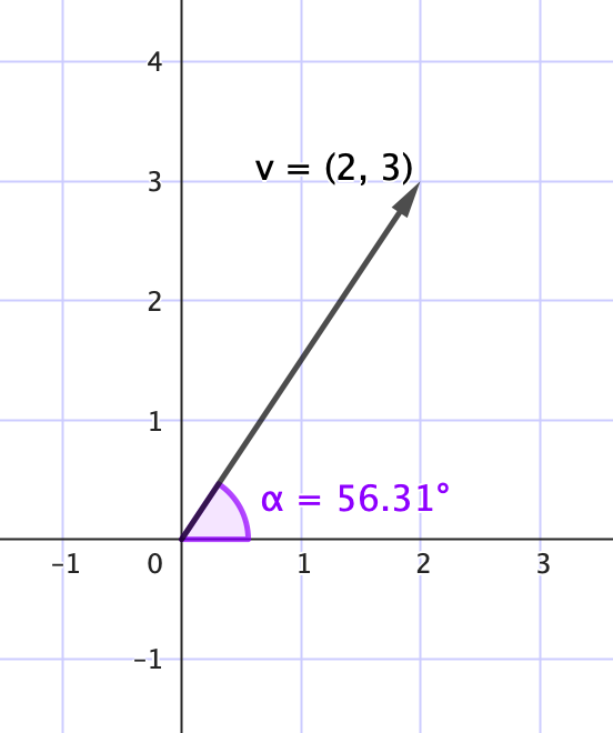
El ángulo de apertura ($\alpha = 56.31^\circ$) indica la dirección del vector respecto al eje horizontal.
donde cada componente $v_i$ representa una cantidad asociada a la categoría $i$, y todas las cantidades se relacionan entre sí. Los vectores también pueden representarse gráficamente como segmentos dirigidos en el plano o el espacio, con magnitud (su tamaño) y una dirección.
Además debemos tener en mente que la norma de un vector se define como
$\|\mathbf{u}\| = \sqrt{u_1^2 + u_2^2 + \cdots + u_n^2}$
y nos sirve, por ejemplo, para calcular el ángulo entre vectores, como se verá más adelante.
Ejemplo
Podemos caracterizar una población de insectos con base en el número de individuos que estás en cada una de las tres etapas del desarrollo característico de este tipo de organismos: huevo (h), larva (l) y adulto (a). Podemos representar el número de individuos en cada etapa como
$$\mathbf{P} = \begin{bmatrix} h \\ l \\ a \end{bmatrix} = \begin{bmatrix} 50 \\ 30 \\ 20 \end{bmatrix}$$
Ejemplo
Se miden tres características de un grupo de plantas: altura (cm), peso (g) y diámetro de flor (mm). Entonces, un vector puede representar un individuo como
$$\mathbf{v} = \begin{bmatrix} \text{cm} \\ \text{g} \\ \text{mm} \end{bmatrix} = \mathbf{v} = \begin{bmatrix} 85 \\ 320 \\ 45 \end{bmatrix}$$
Operaciones básicas con vectores
• Suma de vectores
La suma de dos vectores $\mathbf{u}, \mathbf{v} \in \mathbb{R}^n$ se define por la operación componente a componente
$$\mathbf{u + v} = \begin{bmatrix} u_1 + v_1 \\ u_2 + v_2 \\ \vdots \\ u_n + v_n \end{bmatrix}$$
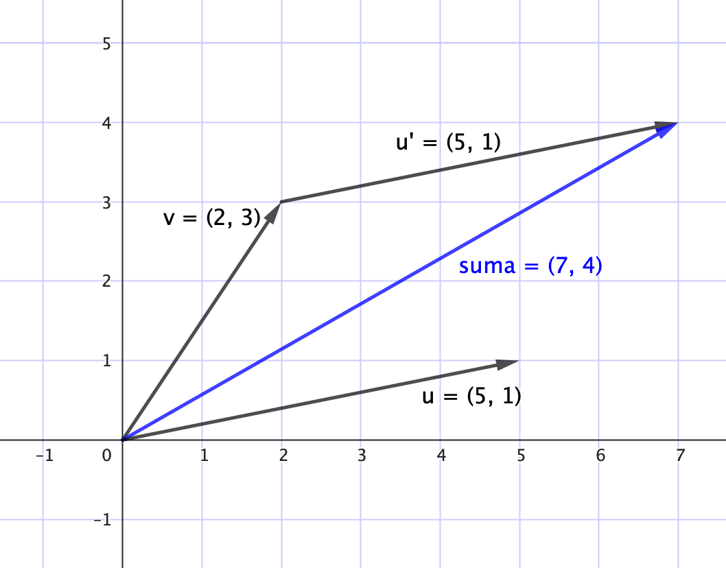
Esta operación es conmutativa y asociativa, lo que permite combinar poblaciones de distintos hábitats o momentos.
Ejemplo
Sean dos poblaciones distintas
$$\mathbf{P_1} = \begin{bmatrix} 5 \\ 8 \\ 2 \end{bmatrix}, \quad \mathbf{P_2} = \begin{bmatrix} 4 \\ 3 \\ 1 \end{bmatrix}$$
La suma será
$$\mathbf{P_1 + P_2} = \begin{bmatrix} 9 \\ 11 \\ 3 \end{bmatrix}$$
lo cual representa la unión de ambas poblaciones por clase.
• Multiplicación por un escalar $\lambda$
La multiplicación de un vector $\mathbf{v}$ por un escalar consiste en multiplicar cada componente del vector por el mismo número real $\lambda$ y se define como
$$\lambda \cdot \mathbf{v} = \begin{bmatrix} \lambda v_1 \\ \lambda v_2 \\ \vdots \\ \lambda v_n \end{bmatrix}$$
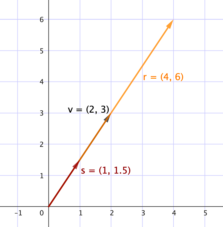
Esta operación modifica la magnitud del vector sin alterar su dirección. Un escalar podría representar una tasa de crecimiento común o una duplicación poblacional por ciclo reproductivo.
Ejemplo
Si una población $\mathbf{P} = \begin{bmatrix} 5 \\ 8 \\ 2 \end{bmatrix}$ se duplica, entonces $\lambda = 2$, luego
$$2 \cdot \mathbf{P} = \begin{bmatrix} 10 \\ 16 \\ 4 \end{bmatrix}$$
Esto representa un crecimiento proporcional en todas las clases.
• Comparación entre vectores: similitud y diferencia
En algunos contextos biológicos se busca saber qué tan similares dos sitios ecológicos, dos comunidades, o dos individuos; y si estos elementos se traducen en vectores, se pueden comparar usando la distancia o el ángulo entre vectores.
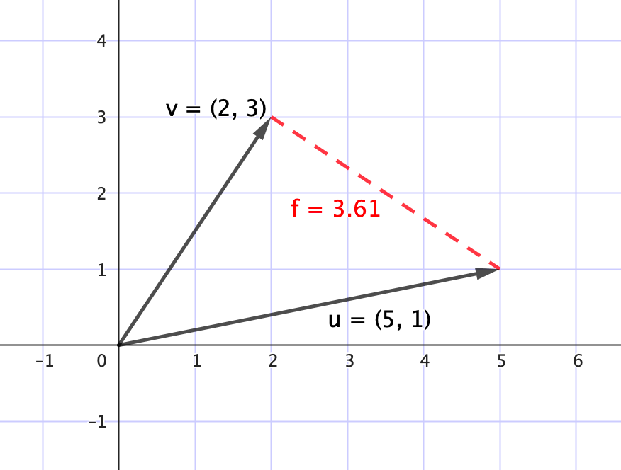
$\qquad$○ Distancia entre vectores
La distancia euclidiana mide la separación entre dos vectores, y se calcula
$d(\mathbf{x}, \mathbf{y}) = \sqrt{(x_1-y_1)^2 + (x_2-y_2)^2 + \cdots + (x_n-y_n)^2}$
De manera que, cuanto mayor sea la distancia, menos similares serán los vectores.
$\qquad$ ○ Ángulo entre vectores
Otra forma de comparar vectores es observando el ángulo que forman entre sí. Podemos calcular el coseno del ángulo entre dos vectores $\mathbf{u}$ y $\mathbf{v}$ como
$\cos(\theta) = \frac{\mathbf{u} \cdot \mathbf{v}}{\|\mathbf{u}\| \cdot \|\mathbf{v}\|}$
donde el producto escalar $\mathbf{u} \cdot \mathbf{v}$ es
$\mathbf{u} \cdot \mathbf{v} = u_1v_1 + u_2v_2 + \cdots + u_nv_n$
De forma que:
$\quad$ □ si $\cos(\theta) = 1$, los vectores tienen la misma dirección (son paralelos);
$\quad$ □ si $\cos(\theta) = 0$, los vectores son ortogonales (forman un ángulo recto);
$\quad$ □ si $\cos(\theta) = -1$, los vectores tienen direcciones opuestas.
Nota: Si el producto escalar es positivo, el ángulo entre los vectores es menor de 90°. Si es negativo, es mayor de 90°. Si es cero, son ortogonales.
• Normalización de un vector y distribución válida
En muchos contextos biológicos necesitamos conocer cómo se reparte el total de individuos entre diferentes clases, especies o estados. Para poder comparar estas estructuras, conviene expresar los valores como proporciones del total. Esta transformación se llama normalización, y consiste en dividir cada componente del vector por la suma total de sus elementos
$\mathbf{v} = \begin{bmatrix} v_1 \\ v_2 \\ \vdots \\ v_n \end{bmatrix} \quad \longrightarrow \quad \hat{\mathbf{v}} = \begin{bmatrix} \frac{v_1}{\sum v_i} \\ \frac{v_2}{\sum v_i} \\ \vdots \\ \frac{v_n}{\sum v_i} \end{bmatrix}$
De esta forma, el vector resultante $\hat{\mathbf{v}}$ representa una distribución de probabilidad discreta, donde cada componente indica la fracción relativa del total.
Es importante no confundir esta normalización (que hace que los componentes sumen 1) con la que convierte a un vector en unitario (es decir, que su norma sea 1).
Además, en este contexto, se dice que un vector es una distribución válida si cumple:
- Todos sus componentes son mayores o iguales a cero: $v_i \geq 0$
- La suma total es igual a 1: $\sum v_i = 1$
En la siguiente liga hay una viñeta de GeoGebra interactiva para visualizar las operaciones de vectores: https://www.geogebra.org/m/zd3hrzxc. Puedes explorar cómo cambian los resultados al modificar las componentes de los vectores.
Ejercicio
Se puede caracterizar una población de peces como estructurada en tres clases etarias (de edades): juveniles (j), adultos (a) y viejos (v). En un año se registraron los siguientes vectores de abundancia de peces por clase en dos lagunas diferentes
$$\mathbf{L_1} = \begin{bmatrix} 25 \\ 40 \\ 10 \end{bmatrix}, \quad \mathbf{L_2} = \begin{bmatrix} 30 \\ 35 \\ 15 \end{bmatrix}$$
a. Responde: ¿cuál laguna presenta una mayor proporción de peces viejos?
b. Calcula la distribución porcentual de cada grupo etario en ambas lagunas.
c. Compara las distribuciones como puntos en el espacio, calcula la distancia entre ellas.
d. (Opcional) Compara las diferencias absolutas entre componentes, luego responde: ¿qué clase muestra mayor diferencia entre lagunas?
Respuesta esperada
a. Laguna 2 tiene más individuos viejos
$$\frac{V}{\text{Total}} = \frac{15}{80} = 18.75\% \quad \text{vs.} \quad \frac{10}{75} = 13.33\%$$
b. Distribuciones porcentuales (normalización)
• Laguna 1
Total = 75
$$\mathbf{\hat{L}_1} = \begin{bmatrix} \frac{25}{75} \ \frac{40}{75} \ \frac{10}{75} \end{bmatrix} = \begin{bmatrix} 0.333 \\ 0.533 \\ 0.133 \end{bmatrix}$$
• Laguna 2
Total = 80
$$\mathbf{\hat{L}_2} = \begin{bmatrix} \frac{30}{80} \ \frac{35}{80} \ \frac{15}{80} \end{bmatrix} = \begin{bmatrix} 0.375 \\ 0.438 \\ 0.188 \end{bmatrix}$$
c.
$\|\hat{\mathbf{L}}_1-\hat{\mathbf{L}}_2\| = \sqrt{(0.333-0.375)^2 + (0.533-0.438)^2 + (0.133-0.188)^2}$
$= \sqrt{(-0.042)^2 + (0.095)^2 + (-0.055)^2} \approx \sqrt{0.0018 + 0.0090 + 0.0030} = \sqrt{0.0138} \approx 0.117$
Se observa una diferencia moderada entre las distribuciones etarias de ambas lagunas.
d. Diferencias absolutas entre componentes:
$\qquad$Juveniles: $|0.333–0.375| = 0.042$
$\qquad$Adultos: $|0.533–0.438| = 0.095$
$\qquad$Viejos: $|0.133–0.188| = 0.055$
Se observa que la mayor diferencia entre lagunas ocurre en los adultos.
Ejercicio
Las densidades relativas (como proporción del total) de tres especies de plantas ($S_1$, $S_2$, $S_3$) en dos sitios diferentes están dadas por los siguientes vectores:
$$\mathbf{x} = \begin{bmatrix} 0.7 \\ 0.2 \\ 0.1 \end{bmatrix}, \quad \mathbf{y} = \begin{bmatrix} 0.5 \\ 0.3 \\ 0.2 \end{bmatrix}$$
a. Suma los vectores y verifica que ambos representan distribuciones válidas.
b. Calcula la distancia entre ambas zonas, luego responde: ¿qué tan diferentes son?
c. Define un vector intermedio $\mathbf{z} = \frac{1}{2}(\mathbf{x} + \mathbf{y})$ y observa si podría representar un sitio de transición ecológica entre las dos zonas.
Respuesta esperada
a. Suma de componentes es
$\qquad \sum \mathbf{x} = 0.7 + 0.2 + 0.1 = 1$
$\qquad \sum \mathbf{y} = 0.5 + 0.3 + 0.2 = 1$
y todos los componentes son mayores que 0.
Luego, ambos son válidos.
b.
$\|\mathbf{x}-\mathbf{y}\| = \sqrt{(0.7 – 0.5)^2 + (0.2 – 0.3)^2 + (0.1 – 0.2)^2} = \sqrt{0.04 + 0.01 + 0.01} = \sqrt{0.06} \approx 0.245$
Se observa que hay una diferencia moderada en composición de especies.
c.
$$\mathbf{z} = \frac{1}{2} \left( \begin{bmatrix} 0.7 \\ 0.2 \\ 0.1 \end{bmatrix} + \begin{bmatrix} 0.5 \\ 0.3 \\ 0.2 \end{bmatrix} \right) = \frac{1}{2} \begin{bmatrix} 1.2 \\ 0.5 \\ 0.3 \end{bmatrix} = \begin{bmatrix} 0.6 \\ 0.25 \\ 0.15 \end{bmatrix}$$
Se observa una mezcla proporcional entre ambas comunidades, lo que puede interpretarse como un ecosistema intermedio en transición.
Ejercicio
Supón que el número de crías que una población genera en cada clase etaria está dado por un vector de fecundidades
$$\mathbf{f} = \begin{bmatrix} 0 \\ 2 \\ 1 \end{bmatrix}$$
y que la estructura actual de la población es
$$\mathbf{P} = \begin{bmatrix} 20 \\ 30 \\ 10 \end{bmatrix}$$
a. Responde: ¿cuántas crías en total se espera que haya en el siguiente ciclo?
b. Reformula el cálculo anterior como un producto escalar y explica la generalización del procedimiento.
c. Interpreta biológicamente qué implicaría que el producto escalar fuera cero.
Respuesta esperada
a. Sólo adultos y viejos se reproducen, por lo que el total de crías sería de $2(30) + 1(10) = 70$
b. El producto escalar es:
$\mathbf{f} \cdot \mathbf{P} = 0(20) + 2(30) + 1(10) = 70$
Si $\mathbf{f}$ representa tasas fecundas por clase, y $\mathbf{P}$ representa estructura poblacional, entonces el producto escalar $\mathbf{f \cdot P}$ representa el número total de crías resultantes.
c. Si $\mathbf{f} \cdot \mathbf{P} = 0$, significaría que ninguna clase tiene fecundidad o no hay individuos en las clases fértiles. En ambos casos, la población no se reproduciría.
Ejercicio
Una especie tiene tres fases de desarrollo: huevo (h), larva (l) y adulto (a). Se sabe que:
• El número de huevos equivale a la suma del doble del número de larvas y del número de adultos.
• La proporción de larvas es igual a la mitad de la de adultos.
• El total de individuos es 112.
a. Calcula cuántos huevos, cuántas larvas y cuántos adultos hay en la población, y escribe el correspondiente vector poblacional $\mathbf{P} = \begin{bmatrix} h \\ l \\ a \end{bmatrix}$.
Respuesta esperada
Se tiene el siguiente sistema:
$$\begin{cases} h = 2a + l \\ l = \frac{1}{2}a \\ h + l + a = 112 \end{cases}$$
Sustituimos
$l = 0.5a \Rightarrow h = 2a + 0.5a = 2.5a$
Luego
$h + l + a = 2.5a + 0.5a + a = 4a = 112 \Rightarrow a = 28$
$l = 14, \quad h = 70$
$\mathbf{P} = \begin{bmatrix} 70 \\ 14 \\ 28 \end{bmatrix}$
Ejercicio
En tres individuos de plantas se miden las características altura (cm) , peso (g), diámetro floral (mm):
$$A= \begin{bmatrix} 90 \\ 300 \\ 45 \end{bmatrix}, \quad B= \begin{bmatrix} 85 \\ 320 \\ 40 \end{bmatrix}, \quad C= \begin{bmatrix} 100 \\ 310 \\ 50 \end{bmatrix}$$
a. Responde: ¿cuál par de individuos es más similar según la distancia euclidiana?
b. Responde: si quieres representar un “individuo promedio”, ¿qué vector usarías?
Respuesta esperada
a.
Distancia A–B:
$\sqrt{(90-85)^2 + (300-320)^2 + (45-40)^2} = \sqrt{25 + 400 + 25} = \sqrt{450} \approx 21.21$
Distancia A–C:
$\sqrt{(90-100)^2 + (300-310)^2 + (45-50)^2} = \sqrt{100 + 100 + 25} = \sqrt{225} = 15.0$
Distancia B–C:
$\sqrt{(85-100)^2 + (320-310)^2 + (40-50)^2} = \sqrt{225 + 100 + 100} = \sqrt{425} \approx 20.62$
Por lo tanto, los individuos A y C son los más similares.
b. Promediamos componente por componente:
$\mathbf{Promedio} = \frac{1}{3} \left( \begin{bmatrix} 90 \\ 300 \\ 45 \end{bmatrix} + \begin{bmatrix} 85 \\ 320 \\ 40 \end{bmatrix} + \begin{bmatrix} 100 \\ 310 \\ 50 \end{bmatrix} \right)$
$\frac{1}{3} \begin{bmatrix} 275 \\ 930 \\ 135 \end{bmatrix} = \begin{bmatrix} 91.67 \\ 310.0 \\ 45.0 \end{bmatrix}$
El individuo promedio tiene: altura ≈ 91.67 cm, peso = 310 g, diámetro floral = 45 mm.
Recursos en línea para profundizar
• Khan Academy – Álgebra vectorial (en español)
https://es.khanacademy.org/math/linear-algebra/vectors-and-spaces
• 3Blue1Brown – Essence of linear algebra (en inglés, visual)
https://www.youtube.com/watch?v=wiuEEkP_XuM&ab_channel=3Blue1BrownEspa%C3%B1ol
• Paul’s Online Math Notes – Vectors
https://tutorial.math.lamar.edu/classes/calcii/vectorsintro.aspx
6.2 Poblaciones estructuradas y sistemas de ecuaciones
Las poblaciones naturales no son homogéneas, los individuos suelen diferenciarse en variables como edad, tamaño corporal, estado fisiológico o reproductivo o condición de salud. Estas diferencias afectan directamente la dinámica de una población. Por ejemplo, no todas las clases de individuos se reproducen o sobreviven igual. Esta diversidad se representa mediante estructura poblacional, que agrupa individuos en clases según variables relevantes.
Para representar cuántos individuos hay en cada clase en un momento dado, usamos un vector poblacional, cuyas componentes —llamadas abundancias— indican el número de individuos en cada clase.
Por ejemplo, si una población de peces se divide en juveniles y adultos, el vector poblacional podría ser
$$\mathbf{x}(t) = \begin{bmatrix} x_1(t) \\ x_2(t) \end{bmatrix} = \begin{bmatrix} \text{número de juveniles en el tiempo } t \\ \text{número de adultos en el tiempo } t \end{bmatrix}$$
La estructura poblacional puede cambiar en el tiempo por eventos como:
• Reproducción: nuevos individuos
• Mortalidad: pérdida de individuos
• Transiciones: migración entre clases
Estas reglas determinan cómo se transforma el vector poblacional de un momentode tiempo $t$ a otro momento $t+k$. En un modelo discreto —por ejemplo, ciclos anuales—, estas transiciones pueden expresarse mediante sistemas de ecuaciones lineales.
Representación matricial de sistemas lineales en modelos poblacionales estructurados
En los modelos de dinámica de poblaciones estructuradas, se estudia cómo cambian con el tiempo las abundancias de distintas clases dentro de una población. Si una población está dividida en $n$ clases, y denotamos por $x_i(t)$ la abundancia de la clase $i$ en el tiempo $t$, entonces el estado poblacional se representa con el vector columna
$$\mathbf{x}(t) = \begin{bmatrix} x_1(t) \\ x_2(t) \\ \vdots \\ x_n(t) \end{bmatrix}$$
El cambio de la población en el tiempo puede describirse mediante un sistema de ecuaciones lineales, donde cada ecuación indica cómo las clases en el tiempo $t$ contribuyen a la formación de una clase específica en el tiempo $t+1$
$$\begin{cases} x_1(t+1) = a_{11}x_1(t) + a_{12}x_2(t) + \cdots + a_{1n}x_n(t) \\ x_2(t+1) = a_{21}x_1(t) + a_{22}x_2(t) + \cdots + a_{2n}x_n(t) \\ \vdots \\ x_n(t+1) = a_{n1}x_1(t) + a_{n2}x_2(t) + \cdots + a_{nn}x_n(t) \end{cases}$$
Cada componente de la matriz $A = [a_{ij}]$ indica cómo la clase $j$ en $t$ contribuye a la clase $i$ en $t+1$. Es decir, las filas corresponden a las clases en el tiempo $t+1$, indican cómo se forma cada clase; las columnas corresponden a las clases en el tiempo $t$, indican de dónde provienen los individuos, luego, las columnas representan la clase de origen y las filas la clase de destino.
Esto permite responder preguntas como ¿Cuántos juveniles habrá el año siguiente?, ¿Qué proporción de adultos actuales se convierten en viejos?, ¿Una clase reproductora es suficiente para mantener la población?
Podemos escribir el sistema en forma matricial como como $\mathbf{x}(t+1) = A \cdot \mathbf{x}(t)$, donde
• $\mathbf{x}(t)$ es el vector poblacional en el tiempo $t$, de tamaño $n \times 1$,
• $A$ es la matriz de transición de tamaño $n \times n$,
• $a_{ij}$ indica cuánto contribuye la clase $j$ en $t$ a la clase $i$ en $t+1$.
Visualmente, esta multiplicación matricial se puede expresar como:
$$\underbrace{ \begin{bmatrix} a_{11} & a_{12} & \cdots & a_{1n} \\ a_{21} & a_{22} & \cdots & a_{2n} \\ \vdots & \vdots & & \vdots \\ a_{n1} & a_{n2} & \cdots & a_{nn} \end{bmatrix} }_{A} \cdot \underbrace{ \begin{bmatrix} x_1(t) \\ x_2(t) \\ \vdots \\ x_n(t) \end{bmatrix} }_{\mathbf{x}(t)} = \underbrace{ \begin{bmatrix} x_1(t+1) \\ x_2(t+1) \\ \vdots \\ x_n(t+1) \end{bmatrix} }_{\mathbf{x}(t+1)}$$
Ejemplo
Consideremos una población dividida en dos clases: $x_1(t)$, juveniles; y $x_2(t)$, adultos.
Las reglas de transición son:
• Cada adulto tiene $b$ crías por ciclo, que al año siguiente pasarán a ser juveniles.
• Una fracción $s$ de los juveniles sobrevive y madura, pasan a ser adultos el año siguiente.
Entonces
$$\begin{cases} x_1(t+1) = b \cdot x_2(t) \\ x_2(t+1) = s \cdot x_1(t) \end{cases}$$
El sistema se puede representar con la matriz $A = \begin{bmatrix} 0 & b \\ s & 0 \end{bmatrix}$ como
$$\mathbf{x}(t+1) = \begin{bmatrix} 0 & b \\ s & 0 \end{bmatrix} \cdot \mathbf{x}(t)$$
En este modelo, el coeficiente $b$ indica el número promedio de crías que produce cada adulto por ciclo (tasa de fecundidad), mientras que $s$ representa la fracción de juveniles que sobreviven y maduran (tasa de maduración).
Ahora, si suponemos que
$\quad$ • $b = 2$ (cada adulto tiene 2 crías)
$\quad$ • $s = 0.5$ (50% de los juveniles maduran)
$\quad$ • el estado inicial es $\mathbf{x}(0) = \begin{bmatrix} 10 \\ 5 \end{bmatrix}$
Entonces tendremos que
$\quad$ • $x_1(1) = 2 \cdot 5 = 10$
$\quad$ • $x_2(1) = 0.5 \cdot 10 = 5$
$\quad$ • $\mathbf{x}(1) = \begin{bmatrix} 10 \\ 5 \end{bmatrix}$
La población regresa exactamente al mismo vector, aunque los individuos nacen, mueren o cambian de clase. Esto ocurre cuando la tasa reproductiva compensa las transiciones exactamente. Sin embargo, esto no significa que el sistema mantenga constante la población para cualquier condición inicial. Por ejemplo, si $\mathbf{x}(0)=\begin{bmatrix}12\\4\end{bmatrix}$, entonces $\mathbf{x}(1)=\begin{bmatrix}8\\6\end{bmatrix},$ y la población total cambia.
Comportamientos posibles de un sistema estructurado
Dependiendo de los valores en la matriz, un sistema puede comportarse de distintas formas a lo largo del tiempo:
1. Estable (equilibrado). El número total de individuos permanece constante a través del tiempo. Esto pasa cuando las reglas de natalidad y transición compensan las pérdidas; cada generación reemplaza a la anterior exactamente. Por ejemplo, una población de aves con natalidad equilibrada.
2. Crecimiento. La población crece indefinidamente. La forma del crecimiento puede ser exponencial o más compleja, pero lo esencial es que cada generación es más numerosa que la anterior. Por ejemplo, una colonia de bacterias en un medio rico para su crecimiento.
3. Extinción. La población disminuye progresivamente hasta desaparecer. Esto pasa cuando las tasas de natalidad y supervivencia son insuficientes para mantener el reemplazo generacional. Por ejemplo, una población aislada y con recursos limitados.
4. Oscilaciones. La población crece y decrece en patrones periódicos. Puede suceder en estructuras de más de dos clases, con rebotes entre fases. Por ejemplo, una población de insectos con fases larva-adulto, donde la reproducción y la maduración producen ciclos.
Ejercicio
Dado el sistema:
$$\mathbf{x}(t+1) = \begin{bmatrix} 0 & 3 \\ 0.4 & 0 \end{bmatrix} \cdot \mathbf{x}(t), \quad \mathbf{x}(0) = \begin{bmatrix} 12 \\ 6 \end{bmatrix}$$
a. Calcula $\mathbf{x}(1)$, $\mathbf{x}(2)$ y $\mathbf{x}(3)$.
b. ¿Qué patrón observas? ¿La población está en equilibrio, crece, decrece, oscila o ninguno de los anteriores?
c. Responde: ¿qué ocurriría si la tasa de maduración cambiara de 0.4 a 0.6?
Respuesta esperada
a.
Cálculo de $\mathbf{x}(1)$
$$\mathbf{x}(1) = A \cdot \mathbf{x}(0) = \begin{bmatrix} 0 & 3 \\ 0.4 & 0 \end{bmatrix} \cdot \begin{bmatrix} 12 \\ 6 \end{bmatrix}$$
$$\Rightarrow \mathbf{x}(1) = \begin{bmatrix} 18 \\ 4.8 \end{bmatrix}$$
Cálculo de $\mathbf{x}(2)$
$$\mathbf{x}(2) = A \cdot \mathbf{x}(1) = \begin{bmatrix} 0 & 3 \\ 0.4 & 0 \end{bmatrix} \cdot \begin{bmatrix} 18 \\ 4.8 \end{bmatrix}$$
$$\Rightarrow \mathbf{x}(2) = \begin{bmatrix} 14.4 \\ 7.2 \end{bmatrix}$$
Cálculo de $\mathbf{x}(3)$
$$\mathbf{x}(3) = A \cdot \mathbf{x}(2) = \begin{bmatrix} 0 & 3 \\ 0.4 & 0 \end{bmatrix} \cdot \begin{bmatrix} 14.4 \\ 7.2 \end{bmatrix}$$
$$\Rightarrow \mathbf{x}(3) = \begin{bmatrix} 21.6 \\ 5.76 \end{bmatrix}$$
b. $\mathbf{x}(2) = \begin{bmatrix} 3 \cdot 4.8 \\ 0.4 \cdot 18 \end{bmatrix} = \begin{bmatrix} 14.4 \\ 7.2 \end{bmatrix}$
Vemos que:
La cantidad de juveniles ($x_1$) sube y baja: 12 → 18 → 14.4 → 21.6
La cantidad de adultos ($x_2$) también varía, no de forma monótona.
Por lo que podemos observar que hay un patrón oscilante. Parece que el sistema rebota entre clases, con aumentos y disminuciones alternadas.
c. En este caso, la matriz sería:
$$A = \begin{bmatrix} 0 & 3 \\ 0.6 & 0 \end{bmatrix}$$
Con una tasa de maduración más alta, más juveniles pasan a adultos cada ciclo. Esto generará más adultos disponibles para reproducirse, lo que a su vez genera más juveniles en el siguiente ciclo. Podríamos decir que este cambio entre clases podría provocar un crecimiento más rápido de la población.
Ejercicio
Supongamos que en una especie de insecto, sólo las larvas son fértiles. Se tiene el sistema:
$$\begin{cases} x_1(t+1) = r \cdot x_1(t) \\ x_2(t+1) = m \cdot x_1(t) \end{cases}$$
donde
$\quad$• $x_1$: larvas (fértiles)
$\quad$• $x_2$: adultos (estériles)
$\quad$• $r$: tasa de reproducción larval
$\quad$• $m$: tasa de maduración
a. Responde: ¿por qué no hay ecuación para $x_2(t)$ contribuyendo a $x_1(t+1)$?
b. Responde: ¿qué tipo de crecimiento tendrá esta población si $r > 1$?
Respuesta esperada
a. Porque los adultos no se reproducen.
b. Crecimiento exponencial (dominancia de larvas).
Ejercicio
Una población se divide en tres clases: A, B y C. Se sabe que:
$\quad$• Cada individuo de C produce 4 nuevos A.
$\quad$• El 50% de los A pasa a B en el siguiente ciclo y el otro 50% permanece en A.
$\quad$• El 30% de los B pasa a C en el siguiente ciclo y el 70% permanece en B.
$\quad$• No hay mortalidad.
a. Construye el sistema de ecuaciones.
b. Escribe la matriz de transición.
c. Con condiciones iniciales $\mathbf{x}(0) = \begin{bmatrix} 40 \\ 0 \\ 0 \end{bmatrix}$, calcula $\mathbf{x}(1)$ y $\mathbf{x}(2)$.
d. (Opcional) Calcula $\mathbf{x}(3)$ y observa lo que sucede.
Respuesta esperada
a. Sean
$\quad$• $x_1(t)$: número de individuos en clase A en el tiempo $t$
$\quad$• $x_2(t)$: número de individuos en clase B
$\quad$• $x_3(t)$: número de individuos en clase C
Entonces
$$\begin{cases} x_1(t+1) = 0.5\,x_1(t) + 4\,x_3(t), \\ x_2(t+1) = 0.5\,x_1(t) + 0.7\,x_2(t), \\ x_3(t+1) = 0.3\,x_2(t). \end{cases}$$
b. La matriz $A$ que representa este sistema es
$$A= \begin{bmatrix} 0.5 & 0 & 4 \\ 0.5 & 0.7 & 0 \\ 0 & 0.3 & 0 \end{bmatrix}$$
Recordemos que las filas describen cómo se forma cada clase en $t+1$, mientras que las columnas representan de qué clase procede cada individuo en el tiempo $t$.
c.
$$\mathbf{x}(1)=A\,\mathbf{x}(0)= \begin{bmatrix} 0.5 & 0 & 4 \\ 0.5 & 0.7 & 0 \\ 0 & 0.3 & 0 \end{bmatrix} \begin{bmatrix} 40 \\ 0 \\ 0 \end{bmatrix} = \begin{bmatrix} 20 \\ 20 \\ 0 \end{bmatrix}$$
La mitad de los individuos en A permanecen ahí, es decir, 20. La otra mitad pasó a B. Aún no hay individuos en C, por lo que no se producen nuevos A.
$$\mathbf{x}(2)=A\,\mathbf{x}(1)= \begin{bmatrix} 0.5 & 0 & 4 \\ 0.5 & 0.7 & 0 \\ 0 & 0.3 & 0 \end{bmatrix} \begin{bmatrix} 20 \\ 20 \\ 0 \end{bmatrix} = \begin{bmatrix} 10 \\ 29 \\ 6 \end{bmatrix}$$
La mitad de los individuos en A que se quedan ahora son 10. Pasan 10 individuos a B, que retiene el 70% (14) y produce el 30% (6) que pasan a C. C sigue sin reproducirse porque recién tiene individuos su clase.
d.
$$\mathbf{x}(3)=A\,\mathbf{x}(2)= \begin{bmatrix} 0.5 & 0 & 4 \\ 0.5 & 0.7 & 0 \\ 0 & 0.3 & 0 \end{bmatrix} \begin{bmatrix} 10 \\ 29 \\ 6 \end{bmatrix} = \begin{bmatrix} 0.5\cdot 10 + 4\cdot 6\\ 0.5\cdot 10 + 0.7\cdot 29 \\ 0.3\cdot 29 \end{bmatrix} = \begin{bmatrix} 34 \\ 23.3 \\ 8.7 \end{bmatrix}$$
Ahora sí hay individuos en C (6), que producen 4 × 6 = 24 nuevos A.