$H$ es semi definida positiva, si $H (x, y) \geq 0 \forall \; (x, y)$
$H$ es semi definida negativa, si $H (x, y) \leq 0 \forall \; (x, y)$
Las formas cuadráticas más fáciles de estudiar son las que tienen asociada una matriz diagonal $$\begin{pmatrix} \lambda_1 & 0 \\ \\ 0 & \lambda_2 \end{pmatrix}$$
Entonces
$$\begin{equation*} H (x, y) = \begin{pmatrix} x & y \end{pmatrix} \begin{pmatrix} \lambda_1 & 0 \\ \\ 0 & \lambda_2 \end{pmatrix} \begin{pmatrix} x \\ y \end{pmatrix} \end{equation*}$$
Si $ (x, y) $ cumple que $ x^2 < y < 3 x^2 $ entonces
$0 < y \, – \, x^2 $ pero $ y \, – \, 3 x^2 < 0 $ por lo tanto $ f (x, y) < 0 $
Si $ (x, y) $ cumple que $ y > 3 x^2 $ entonces $ f (x, y) > 0 $ ya que $ y > x^2$
En el siguiente enlace puedes ver la gráfica de la función $f(x,y) = ( y \, – \, 3x^2) ( y \, – \, x^2)$ y de la curva de nivel $ ( y \, – \, 3x^2) ( y \, – \, x^2) = 0$.
Como ya podrás haber notado, identificar la compacidad en un espacio métrico es una situación recurrente y de interés en cursos de Análisis. Naturalmente han surgido resultados que permiten identificarla con mayor facilidad en conjuntos cuya métrica no es tan sencilla de manejar, como los espacios de funciones.
En esta entrada veremos un teorema útil para trabajar en el espacio $\mathcal{C^0}(X,Y)$ donde $X$ es compacto y $Y$ es completo. Primero veamos si el siguiente conjunto de funciones es compacto.
Para cada $n \in \mathbb{N}$ considera la función $f_n:[0,2] \to \mathbb{R}$ dada por
La familia de funciones $\mathcal{H}:= \{f_i \, | \, i \in \mathbb{N}\}$ no es compacta en el espacio $\mathcal{C}^0[0,2]$ porque no es totalmente acotada: Es sencillo ver que para cualesquiera dos funciones $f_l, f_m \in \mathcal{H}$ con $l \neq m,$ se cumple que $d_{\infty}(f_l,f_m)=1.$ De modo que no es posible cubrir $\mathcal{H}$ con una cantidad finita de bolas abiertas de radio $\frac{1}{2}.$ Esto se debe a que cualquier bola abierta $B(f, \frac{1}{2}) \subset \mathcal{C}^0[0,2]$ tiene a lo más un elemento de $\mathcal{H}:$ Si $f_l, f_m \in B(f, \frac{1}{2})$ se cumple que $d_{\infty}(f_l,f_m) \leq d_{\infty}(f_l,f)+d_{\infty}(f,f_m) < \frac{1}{2}+\frac{1}{2}= 1$ lo cual es una contradicción a la distancia entre ambas funciones. En consecuencia no será posible cubrir todos los elementos de $\mathcal{H}$ con una cantidad finita de bolas por lo que $\mathcal{H}$ no será totalmente acotado.
Las características de esta familia de funciones nos impiden «atraparlas» en bolitas pequeñitas. Como la distancia entre funciones está en función de las distancias en puntos del codominio, necesitaremos propiedades que restrinjan el comportamiento de alguna manera. Una propiedad que lo logra es, como vimos en la entrada anterior, la equicontinuidad en funciones. Puedes observar que $\mathcal{H}$ no es equicontinua, pues para $\varepsilon = \frac{1}{2}$ no existe ningún valor de $\delta$ que funcione. Conforme $n \to \infty$ la gráfica de las funciones genera un pico que sube y baja rápidamente en un intervalo, de tamaño $\frac{2}{n^2},$ que también se va haciendo más pequeño. Siempre será posible elegir una función donde el tamaño del intervalo es menor que $\delta.$ Habrá un punto $x$ tal que $|x- \frac{1}{n}|< \delta$ pero $|f(x)-f(\frac{1}{n})| =|0-1|=1> \frac{1}{2}.$
¿Bastará la equicontinuidad de una familia de funciones para que esta sea compacta? No es así. Presentamos una familia de funciones equicontinuas que no es totalmente acotada.
Para cada $n \in \mathbb{N}$ y $x \in [0,1]$ sea $f_n(x):= e_n,$ donde $e_n$ es la sucesión que toma valor $1$ en la entrada i-ésima y $0$ en el resto. Entonces la familia $\mathcal{H}:= \{f_n \, | \, n \in \mathbb{N}\}$ es equicontinua pues, para todo $\varepsilon >0,$ (sin importar el valor de $\delta),$ para cualesquiera $x,y \in [0,1]$ se cumplirá para cualquier $f_n \in \mathcal{H}$ que $\norm{f_n(x)-f_n(y)}_2= \norm{e_n-e_n}_2 = 0 < \varepsilon.$
No obstante, esta familia no es totalmente acotada: Para cualesquiera dos funciones en $\mathcal{H},$ digamos $f_l, f_m, l \neq m$ tenemos que $d_{\infty}(f_l,f_m) = \norm{e_l-e_m}_2 = \sqrt{|1|^2+|1|^2} = \sqrt{2}.$ En consecuencia, no será posible cubrir $\mathcal{H}$ con una cantidad finita de bolas abiertas de radio $\frac{\sqrt{2}}{2}$ por lo que esta familia no es totalmente acotada.
Esta vez no bastó la equicontinuidad, incluso con funciones tan «estables» que son constantes. La falla radicó en que, al variar la función en la que evaluamos un punto $x$ del dominio, el conjunto dado por las imágenes de $\{x\}$ no es relativamente compacto.
Ahora veremos las condiciones necesarias y suficientes que debe tener una familia de funciones para ser relativamente compacta:
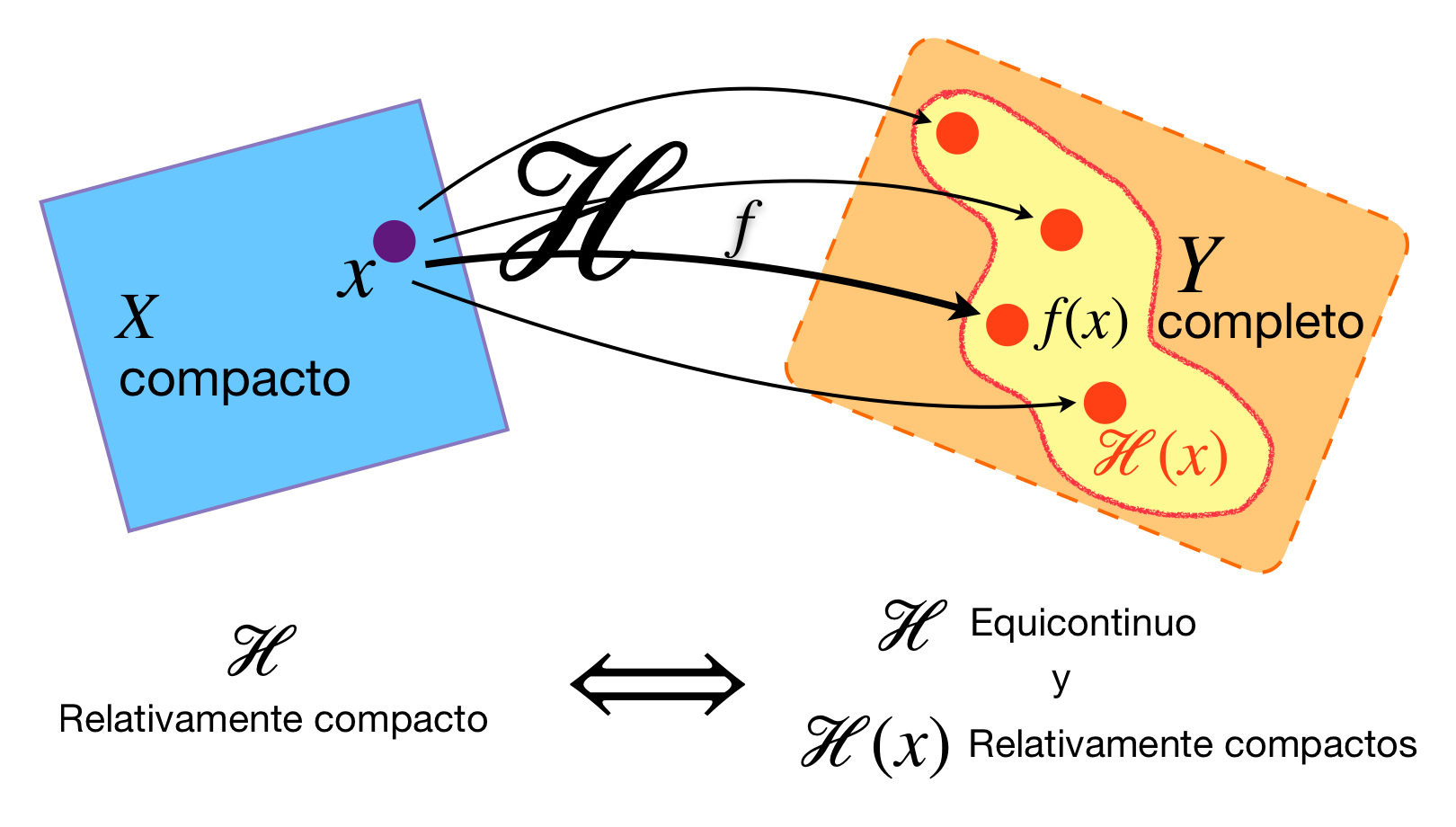
Teorema Arzelá-Ascoli. Sean $X$ un espacio métrico compacto y $Y$ un espacio métrico completo. Un subconjunto $\mathcal{H}$ de $\mathcal{C^0}(X,Y)$ es relativamente compacto en el espacio $\mathcal{C^0}(X,Y)$ si y solo si $\mathcal{H}$ es equicontinuo y los conjuntos definidos como $\mathcal{H}(x):= \{f(x) \, | \, f \in \mathcal{H}\}$ son relativamente compactos en $Y$ para cada $x \in X.$
Representación del teorema de Arzelá-Ascoli.
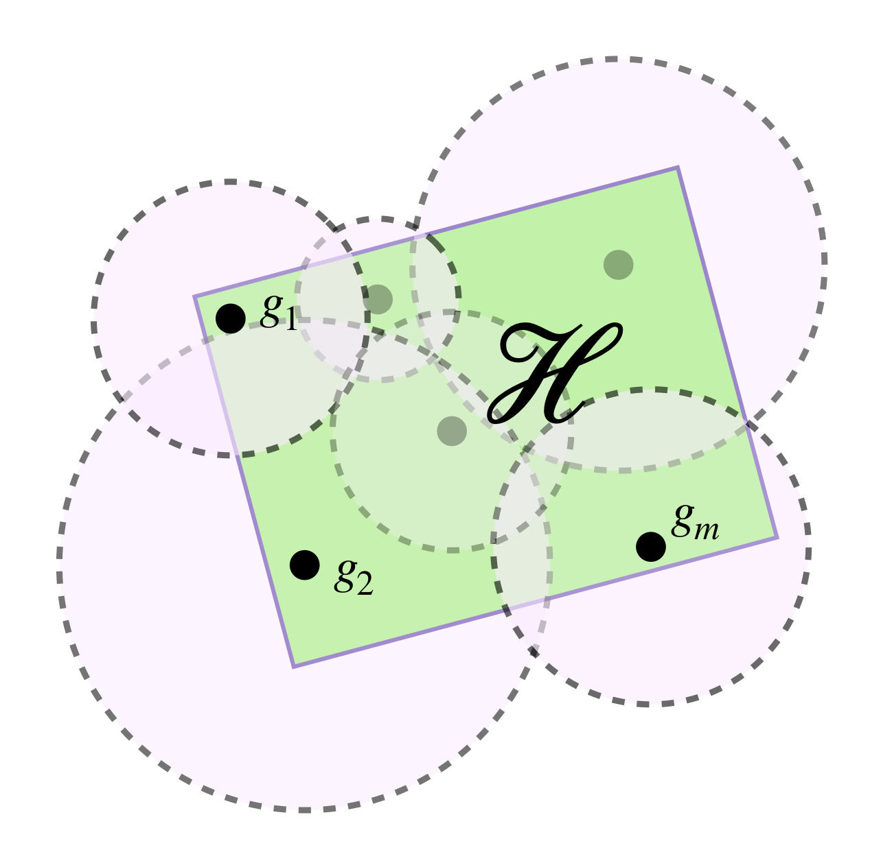
Demostración: En Convergencia uniforme y continuidad concluimos que por las propiedades de $X$ y $Y, \,$ $\mathcal{C^0}(X,Y)$ es completo, así por lo visto en conjuntos relativamente compactos y totalmente acotados sabemos que como $\mathcal{H}$ es relativamente compacto en $\mathcal{C^0}(X,Y),$ esto implica que $\mathcal{H}$ es totalmente acotado. Sea $\varepsilon >0.$ Existen funciones $g_1, \, g_2,…,g_m \in \mathcal{H}$ tales que \begin{align} \mathcal{H} \subset B_\infty \left(g_1, \, \frac{\varepsilon}{3} \right) \cup B_\infty \left(g_2, \, \frac{\varepsilon}{3} \right) \cup … \cup B_\infty \left(g_m, \, \frac{\varepsilon}{3} \right). \end{align} Donde $B_\infty$ denota bolas abiertas con la métrica uniforme en $\mathcal{C^0}(X,Y)$
En el dibujo las $g’s $ aunque son puntos representan funciones. La zona verde es el conjunto de funciones $\mathcal{H}.$ Las bolas abiertas descritas lo cubren.
Esto significa que cualquier función de $\mathcal{H}$ se aproxima mucho a alguna $g_i, \, i \in \{1,2,..,m\}.$ Sea $x \in X.$ Considera el conjunto $$\mathcal{H}(x):= \{f(x) \, | \, f \in \mathcal{H}\}$$
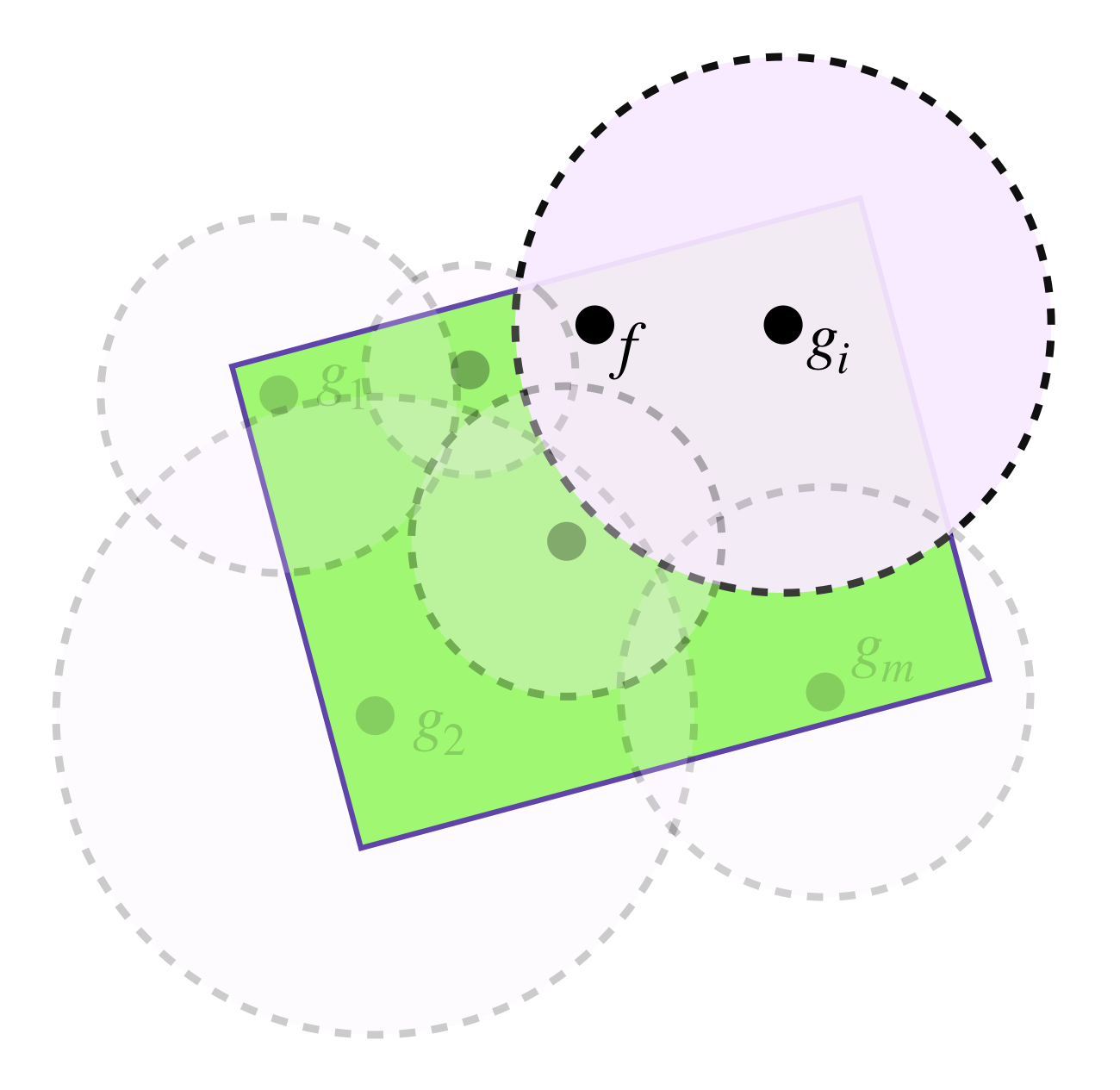
La función $f$ es elemento de alguna de las bolas abiertas que cubren a $\mathcal{H}.$
Dado un $f(x) \in \mathcal{H}(x),$ por (1) sabemos que existe $i \in \{1,2,..,m\}$ tal que la función $f \in B_\infty \left(g_i, \, \frac{\varepsilon}{3} \right).$
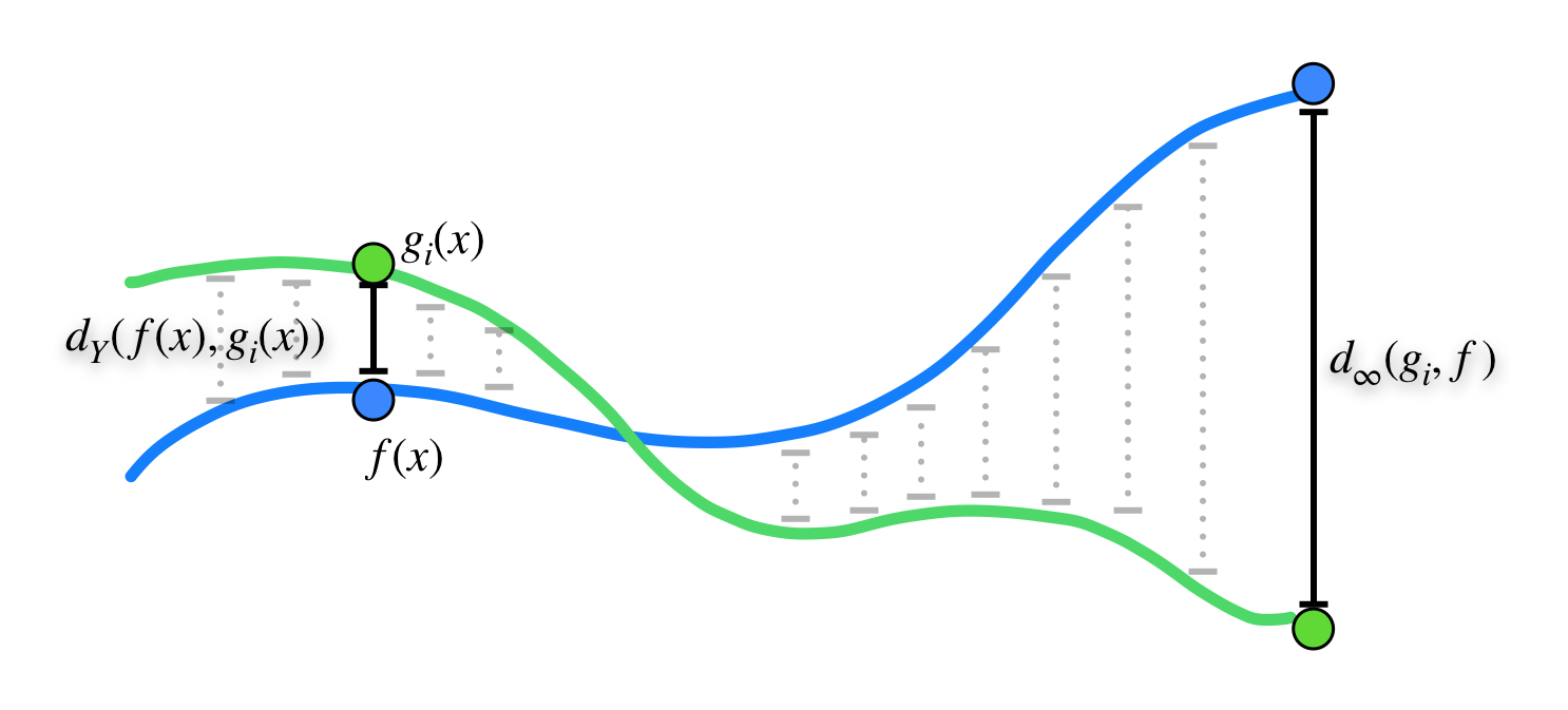
La distancia entre dos puntos $f(x)$ y $g_i(x)$ es menor igual que la distancia entre ambas funciones.
De modo que $d_\infty (g_i,f) < \frac{\varepsilon}{3}. $ En particular para $x$ se cumple que $d_Y(g_i(x),f(x)) < \frac{\varepsilon}{3}$ por lo tanto $$f(x) \in B_Y \left( g_i(x), \, \frac{\varepsilon}{3} \right)$$
De donde se sigue \begin{align} \mathcal{H}(x) \subset B_Y \left( g_1(x), \, \frac{\varepsilon}{3} \right) \cup B_Y \left( g_2(x), \, \frac{\varepsilon}{3} \right) \cup … \cup B_Y \left( g_m(x), \, \frac{\varepsilon}{3} \right) \end{align} lo que significa que $\mathcal{H}(x)$ es totalmente acotado. Como $Y$ es completo se sigue por la equivalencia de conjuntos relativamente compactos y totalmente acotados que $\mathcal{H}(x)$ es relativamente compacto en $Y.$
Para probar que $\mathcal{H}$ es equicontinuo tomemos en cuenta que $X$ es compacto y por lo visto en la entrada Continuidad uniforme sabemos que cada $g_i$ es uniformemente continua en $X.$ Entonces cada $g_i$ tiene su respectiva $\delta_i >0$ tal que para cualesquiera $x,z \in X,$ si $d_X(x,z)< \delta_i$ entonces $$d_Y(g_i(x),g_i(z)) < \frac{\varepsilon}{3.}$$
Sea $\delta := min \{\delta_1,…,\delta_m\}.$ Sea $f \in \mathcal{H}.$ Dicho lo anterior y recordando que existe $i \in \{1,2,..,m\}$ tal que $f \in B_\infty \left(g_i, \, \frac{\varepsilon}{3} \right),$ tenemos que si $d_X(x,z) < \delta$ entonces
Acontinuación probaremos el regreso. Tengamos presentes las ideas: suponemos que $\mathcal{H}$ es equicontinuo y para cada $x \in X,$ los conjuntos definidos como $\mathcal{H}(x):= \{f(x) \, | \, f \in \mathcal{H}\}$ son relativamente compactos en $Y.$ Buscamos demostrar que $\mathcal{H}$ de $\mathcal{C^0}(X,Y)$ es relativamente compacto en el espacio $\mathcal{C^0}(X,Y).$
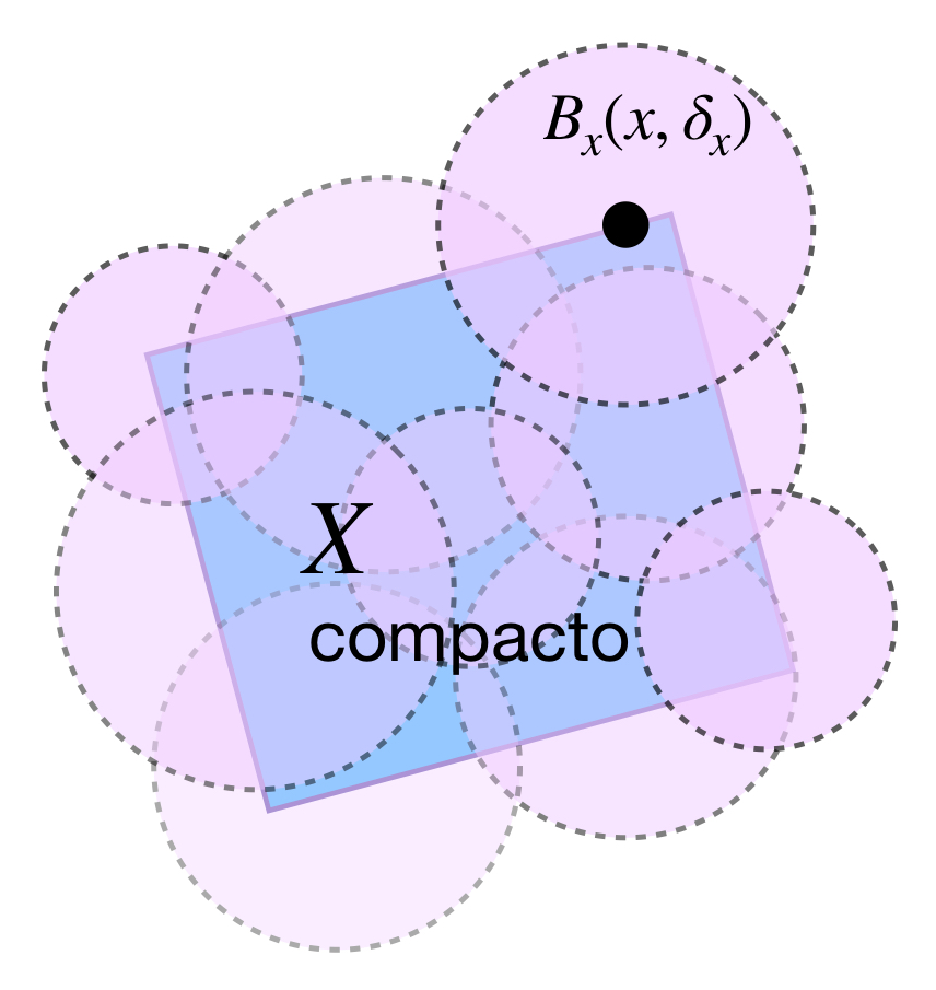
Sea $\varepsilon >0.$ Como $\mathcal{H}$ es equicontinuo, para cada $x \in X$ existe $\delta_x >0$ tal que para toda $f \in \mathcal{H}$ siempre que $d_X(x,z) < \delta_x,$ con $z \in X,$ se satisface \begin{align} d_Y(f(z),f(x)) < \frac{\varepsilon}{4} \end{align}
Por supuesto que $\{B_X \left( x, \delta_x \right) \, | \, \, x \in X \}$ es una cubierta abierta de $X.$
$X$ cubierto por bolas abiertas con centro en cada punto de $X.$
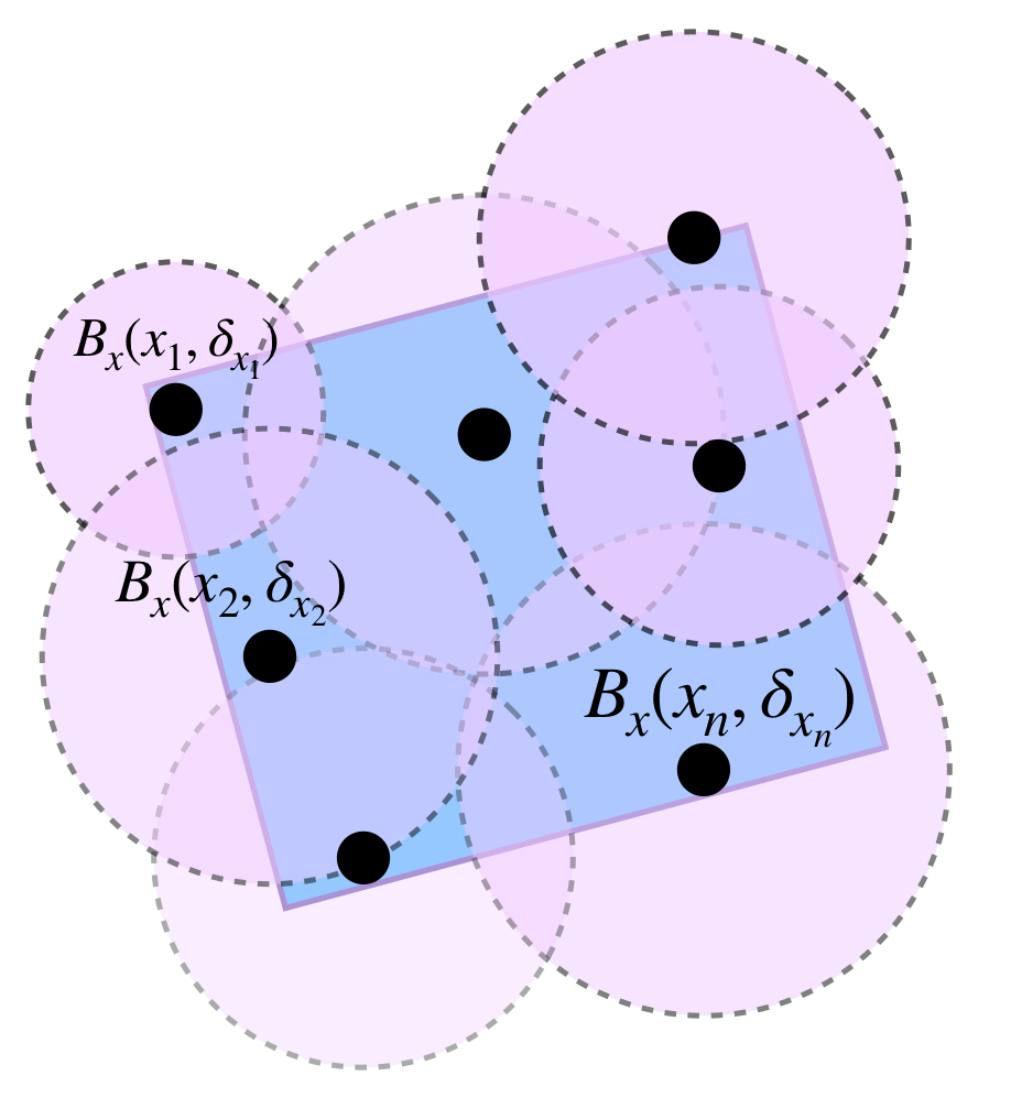
Como es compacto, existen $x_1, \, x_2,…,x_n \, \in X$ tales que
$X$ cubierto por una cantidad finita de esas bolas.
y como cada $\mathcal{H}(x_i), \, i \in \{1,…,n\}$ es totalmente acotado, para cada $x_i$ existen $y^i_1,\ y^i_2,…,y^i_{k_i} \, \in Y$ tales que \begin{align} \mathcal{H}(x_i) \subset B_Y \left( y^i_1, \frac{\varepsilon}{4} \right) \cup B_Y \left( y^i_2, \frac{\varepsilon}{4} \right) \cup… \cup B_Y \left( y^i_{k_i}, \frac{\varepsilon}{4} \right) \end{align}
Uniendo todos los $\mathcal{H}(x_i)$ y todas las bolas que cubren a estos conjuntos tenemos que, renombrando los centros, existen finitos $y_1,…,y_{m} \, \in Y$ que satisfacen
Podemos pensar en clasificar las funciones de $\mathcal{H}$ dependiendo de a qué bola de radio $y_k,$ para algún $k \in \{1,…,m\}$ es enviado cada $x_i, \, i \in \{1,…,n\}.$ Como este comportamiento puede asignarse a través de una función $\sigma:\{1,2,…,n\} \to \{1,2,…,m\},$ definimos los conjuntos:
Argumentando formalmente, si $f \in \mathcal{H}$ por la expresión (7) se asegura que cada $f(x_i)$ con $i \in \{1,2,…,n\}$ está en alguna bola $B_Y \left( y_k, \frac{\varepsilon}{4} \right)$ para algún $k \in \{1,2,…,m\}.$ Nota que la función que relaciona a cada $i$ con su respectiva $k,$ según esta descripción, es algún elemento $\sigma \in S,$ por lo tanto se cumple (8).
Ahora vamos a probar que cada $\mathcal{H}_\sigma$ está contenida en una bola de radio $\varepsilon$ con centro en $\mathcal{H}.$
Considera $f,g \in \mathcal{H}_\sigma$ y sea $x \in X.$ Por (5) $x$ pertenece a alguna bola abierta $B_X(x_i, \delta_{x_i})$ para algún $i \in \{1,2,…,n\}.$ Entonces $d_X(x,x_i)< \delta_{x_i}.$ Recordemos que esta $\delta_{x_i}$ se eligió de tal forma que satisface la definición de equicontinuidad en $x_i.$ Así, según (4) se sigue que para cada $h \in \mathcal{H}:$ $$d_Y(h(x),h(x_i)) < \frac{\varepsilon}{4}.$$
Si tomamos el máximo de las $x´s \in X$ concluimos que $d_\infty(f,g) < \varepsilon$ para cualesquiera $f,g \in \mathcal{H}_\sigma,$ en consecuencia el conjunto $\mathcal{H}_\sigma$ está contenido en una bola de radio $\varepsilon$ con centro en cualquiera de sus funciones. Es decir, para cualquier $g_\sigma \in \mathcal{H}_\sigma$
Y como $S$ es finito, concluimos que $\mathcal{H}$ es totalmente acotado.
Terminemos esta sección con el siguiente:
Corolario. Sea $X$ un espacio métrico compacto. Un subconjunto $\mathcal{H}$ de $\mathcal{C}^0(X, \mathbb{R}^n)$ es relativamente compacto en $\mathcal{C}^0(X, \mathbb{R}^n)$ si y solo si $\mathcal{H}$ es equicontinuo y acotado en $\mathcal{C}^0(X, \mathbb{R}^n).$
Demostración: Sea $\mathcal{H}$ un subconjunto relativamente compacto en $\mathcal{C}^0(X, \mathbb{R}^n).$ Por el teorema de Arzelá-Ascoli, $\mathcal{H}$ es equicontinuo. Como $\overline{\mathcal{H}}$ es compacto entonces es acotado en $\mathcal{C}^0(X, \mathbb{R}^n),$ por lo tanto $\mathcal{H}$ también es acotado en $\mathcal{C}^0(X, \mathbb{R}^n).$
Ahora supongamos que $\mathcal{H}$ es equicontinuo y acotado en $\mathcal{C}^0(X, \mathbb{R}^n).$ Entonces existen $f_0 \in \mathcal{H}$ y $M>0$ tales que para cada $f \in \mathcal{H}$
De aquí podemos concluir que para cada $x \in X,$ el conjunto $\mathcal{H}(x)$ está acotado en $\mathbb{R}^n$ entonces así lo es también su cerradura, por lo que $\overline{\mathcal{H}}$ es cerrado y acotado en $\mathbb{R}^n$ de modo que $\mathcal{H}(x)$ es relativamente compacto y por el teorema de Arzelá-Ascoli, se cumple que $\mathcal{H}$ es relativamente compacto en $\mathcal{C}^0(X, \mathbb{R}^n).$
Más adelante…
Terminaremos la sección de compacidad mostrando un concepto que sigue la misma idea de las bolas de radio $\varepsilon$ que son las $\varepsilon$-redes. Hablaremos de la métrica de Hausdorff y de cómo es posible entender la compacidad a través de conjuntos finitos.
Tarea moral
Para cada $n \in \mathbb{N},$ sea $f_n:[0, \infty) \to \mathbb{R}$ tal que $f_n(x):= sen \sqrt{x + 4 \pi ^2 n ^2}.$ Demuestra que a) El conjunto $\mathcal{H} := \{f_n \, | \, n \in \mathbb{N} \}$ es equicontinuo. b) Para cada $x \in [0, \infty)$ el conjunto $\mathcal{H}(x)$ es relativamente compacto en $\mathbb{R}.$ Te sugerimos probar que la sucesión $(f_n)_{n \in \mathbb{N}}$ converge puntualmente a $0$ en $[0, \infty).$ c) $\mathcal{H}$ no es un subconjunto compacto de $\mathcal{C}_b ^0([0, \infty), \mathbb{R}).$ Te sugerimos probar que la sucesión $(f_n)_{n \in \mathbb{N}}$ no converge uniformemente a $0$ en $[0, \infty).$ Concluye que la compacidad de $X$ es necesaria en el teorema de Arzelá-Ascoli.
Sea $X := \{ (x,y) \in \mathbb{R}^2 \, | \, (x,y) \neq (\frac{1}{2},0) \}$ y sea $f_n \in \mathcal{C}^0([0,1],X)$ tal que $f_n(x) := (x, \frac{1}{n} sen \pi x).$ Considera el conjunto $\mathcal{H} := \{f_n \, | \, n \in \mathbb{N}\}.$ a) ¿Es $\mathcal{H}$ equicontinuo? b) ¿Es $\mathcal{H}$ acotado en $\mathcal{C}^0([0,1],X)?$ c) ¿Es $\mathcal{H}$ relativamente compacto en $\mathcal{C}^0([0,1],X)?$
5.4 El demonio de Laplace y el fin de la infancia: sensibilidad a las condiciones iniciales, bifurcaciones y caos
A lo largo de este bloque hemos trabajado con modelos matemáticos que podrían haberte dado la impresión de que el futuro de un sistema es completamente predecible. Damos una condición inicial, aplicamos una regla o fórmula (por ejemplo, el modelo logístico o el de Malthus), y obtenemos una secuencia de valores que muestran cómo evoluciona una población a lo largo del tiempo. Este proceso sugiere que, si conocemos suficientemente bien cómo funciona un sistema y con qué valores iniciales comenzamos, podríamos predecir su comportamiento futuro con exactitud. Pero, ¿es realmente así como sucede?
Esta noción no es nueva. A comienzos del siglo XIX, el matemático y filósofo Pierre-Simon Laplace propuso una idea que, en su momento, se volvió tendencia en la comunidad científica: imaginen una inteligencia capaz de conocer absolutamente todas las leyes de la naturaleza y la posición de cada partícula del universo en un momento dado. Esa inteligencia, conocida como el demonio de Laplace, podría predecir el futuro con total certeza, ya que todo el universo seguiría un comportamiento determinista, todo lo que ocurre está determinado por lo que ocurrió antes.
Es importante aclarar que Laplace nunca utilizó la figura del demonio de manera explícita en sus escritos, este concepto fue popularizado por filósofos y científicos posteriores. En su Essai philosophique sur les probabilités (1814), Laplace especuló sobre un universo gobernado por el determinismo absoluto:
“Podemos considerar el estado actual del universo como el efecto de su pasado y la causa de su futuro. Un intelecto que, en cualquier momento dado, conociera todas las fuerzas que animan la naturaleza y las posiciones mutuas de los seres que la componen, si este intelecto fuera lo suficientemente vasto como para someter los datos a análisis, podría condensar en una sola fórmula el movimiento de los cuerpos más grandes del universo y el del átomo más ligero; para tal intelecto nada sería incierto y el futuro, al igual que el pasado, estaría presente ante sus ojos.”
Esta idea, aunada a la mecánica Newtoniana, tuvo una fuerte influencia, muchos científicos creyeron que la naturaleza, al igual que una máquina de relojería, podría ser comprendida de manera determinista. De acuerdo con esta visión, si pudiéramos medir con precisión todas las condiciones iniciales, podríamos predecir el futuro con exactitud. A continuación vamos a considerar la complejidad de los sistemas no lineales, como los que encontramos en la biología y en otros sistemas dinámicos.
El fin de la infancia: cuando el orden se vuelve caótico
A mediados del siglo XX, se comenzó a investigar lo que sucede en sistemas no lineales, como el modelo logístico que ya hemos visto en este curso. Lo que descubrieron es que, para ciertos valores de los parámetros, pequeñas diferencias en las condiciones iniciales pueden llevar a resultados completamente distintos después de varias iteraciones. Este fenómeno se conoce como sensibilidad a las condiciones iniciales. Como explica Robert May (1976), incluso modelos tan simples como el logístico pueden mostrar un comportamiento caótico.
Veamos un ejemplo sencillo. Supongamos que usamos el modelo logístico que ya hemos trabajado:
$x_{n+1} = r x_n (1 – x_n)$
Y elegimos un valor de r = 3.9, con dos condiciones iniciales muy cercanas: $x_0 = 0.500$ y $x_0 = 0.501$. Si calculamos las siguientes generaciones, al principio los resultados de $x_n$ pueden parecer muy similares, pero después de unas cuantas iteraciones, las diferencias entre ambos valores se amplifican hasta que parecen completamente distintas. Esto significa que, aunque el modelo es determinista (es decir, no tiene ninguna parte aleatoria), es tan sensible a los valores iniciales que el resultado final no es predecible con certeza. Este comportamiento se llama caos determinista, y aunque el término caos se suele asociar con desorden, en este contexto se refiere a un tipo de orden muy complejo, pero impredecible a largo plazo.
Y esto, ¿qué tiene que ver con la biología?
Algunos modelos muestran sensibilidad a las condiciones iniciales, incluso aquellos que pueden comportarse de manera determinista para ciertos parámetros, con otros ligeramente diferentes pueden mostrar caos. Esto significa que una ligera variación en factores como la tasa de crecimiento, la disponibilidad de recursos o la proporción de individuos de una especie puede cambiar completamente las predicciones del modelo.
Para mostrar lo que ligeras variaciones en los parámetros de un sistema pueden ocasionar, revisar el ejemplo gráfico del subtema 5.3, en https://www.geogebra.org/m/wpurkns6 puedes encontrar la construcción del ejemplo mencionado.
A pesar de que los modelos matemáticos son herramientas importantes y muy útiles, la predicción exacta en biología es extremadamente difícil. En la mayoría de los casos, no se trata de predecir con certeza lo que sucederá, sino de entender las posibles trayectorias y comportamientos del sistema. Los modelos nos permiten explorar diferentes escenarios y conocer qué podría suceder bajo ciertas condiciones, pero las predicciones precisas, especialmente a largo plazo, son prácticamente imposibles.
Como reflexionó Ian Stewart (Stewart, I., 1989), la aparición del concepto del caos determinista representa el fin de la inocencia del pensamiento científico, es el momento en el que dejamos de creer que todo puede preverse y comenzamos a aceptar que la naturaleza no sigue caminos predecibles, sino que siempre tiene comportamientos inesperados. Es esencial comprender y ser conscientes de las limitaciones al usar modelos matemáticos, así como tener en cuenta que nuestras mediciones son aproximadas, y que los resultados pueden verse influenciados por factores que no hemos considerado en el modelo.
5.5 Otros sistemas dinámicos en tiempo discreto: ley del equilibrio de Hardy-Weinberg. Modelos de selección natural
Hasta ahora hemos estudiado cómo algunos modelos pueden describir la evolución de una población a lo largo del tiempo: cómo crece, cómo se estabiliza o incluso cómo cambia drásticamente dependiendo de sus condiciones iniciales. En este subtema aplicaremos ideas similares al estudio de la genética de poblaciones, es decir, a cómo cambian las frecuencias de alelos y genotipos a través de las generaciones.
En este contexto, nos enfocaremos en un caso particular que funciona como punto de partida en genética poblacional: el modelo de equilibrio de Hardy-Weinberg. Este modelo no describe el cambio, sino la ausencia de cambio, y establece las condiciones bajo las cuales se espera que las frecuencias genéticas se mantengan constantes generación tras generación. Sirve, por tanto, como modelo nulo para evaluar si hay o no fuerzas evolutivas actuando sobre una población.
¿Qué es una hipótesis nula?
Se trata de una suposición base en un análisis científico que plantea que no hay efecto significativo entre las variables que se estudian. En genética, la hipótesis nula suele ser que las frecuencias alélicas y genotípicas no están cambiando en la población.
El equilibrio de Hardy-Weinberg representa justamente esta hipótesis nula. Según este modelo, si no hay selección natural, mutación, migración, deriva genética ni apareamiento no aleatorio, las frecuencias de los alelos y de los genotipos permanecerán estables de una generación a otra. Cualquier desviación entre lo que predice el modelo y lo que se observa en la realidad sugiere que alguna fuerza evolutiva podría estar actuando.
El modelo de Hardy-Weinberg
Este modelo establece que, en una población ideal, las frecuencias esperadas de los alelos y los genotipos permanecen constantes de una generación a otra si se cumple las siguientes condiciones: $\quad$• Población de tamaño muy grande (sin deriva genética). $\quad$• Apareamiento aleatorio (sin selección sexual). $\quad$• Ausencia de selección natural. $\quad$• Ausencia de mutaciones. $\quad$• Ausencia de migración (flujo génico).
Bajo estos supuestos, se generan expectativas sobre cómo deberían distribuirse los genotipos. Para una población con dos alelos, $A$ y $a$: $\quad$Sea $p$ la frecuencia relativa del alelo $A$, $\quad$sea $q$ la frecuencia relativa del alelo $a$, $\quad$como sólo hay dos alelos, $p+q=1$, luego $q=1-p$.
Las frecuencias genotípicas en equilibrio se calculan: $\quad$Frecuencia del genotipo AA: $f_{AA} = p^2$ $\quad$Frecuencia del genotipo Aa: $f_{Aa} = 2pq$ $\quad$Frecuencia del genotipo aa: $f_{aa} = q^2$
Si suponemos que hay una población con datos genotípicos observados. Para saber si está en equilibrio: $\quad$1. Calculamos p y q a partir de los datos observados, por ejemplo, si se conocen los genotipos $AA$, $Aa$ y $aa$: $$p = \frac{2 \times (\text{número de individuos AA}) + (\text{número de individuos Aa})}{2 \times (\text{número total de individuos})}$$
2. Calculamos las frecuencias esperadas $p^2$, $2pq$, $q^2$. 3. Comparamos con los valores observados usando una prueba como chi-cuadrada: $$\chi^2 = \sum \frac{(O_i – E_i)^2}{E_i}$$ donde $O_i$ y $E_i$ son los valores observados y esperados para cada genotipo. 4. La aptitud puede verse como la probabilidad de que ese genotipo contribuya descendencia a la siguiente generación. Para calcular la frecuencia del alelo $A$ en la siguiente generación, usamos esta fórmula:
Donde $\overline{w}$ es la aptitud media de la población: $\overline{w} = p^2 w_{AA} + 2pq w_{Aa} + q^2 w_{aa}$
Guía rápida de prueba chi-cuadrada
1. Obtener el número de individuos para cada genotipo y el tamaño total de la muestra (N). 2. Calcular $p$ y $q$ a partir de los datos observados. 3. Calcular $p^2$, $2pq$, $q^2$ y multiplica cada frecuencia por $N$ para obtener las frecuencias esperadas. 3. Aplicar la fórmula de chi-cuadrada: $\chi^2 = \sum \frac{(O_i – E_i)^2}{E_i}$ 4. Determinar los grados de libertad (gl): gl = número de clases – número de parámetros estimados – 1 (p. e. supongamos que hay 3 genotipos (AA, Aa, aa), luego, hay 3 clases; y hay 1 parámetro estimado que es la frecuencia alélica $p$. Entonces: gl = 3 – 1 – 1 = 1) 5. Comparar con $\chi^2$ crítico, que es un número usado como umbral para decidir si la diferencia observada es significativa o no. Una vez calculado $\chi^2$, se compara con el valor crítico correspondiente al número de grados de libertad.
gl
1
2
3
Valor crítico (α = 0.05)
3.841
5.991
7.815
$\quad$• Si $\chi^2 > \chi^2_{\text{crítico}}$: se rechaza la hipótesis nula → hay evidencia de que no hay equilibrio. $\quad$• Si $\chi^2 < \chi^2_{\text{crítico}}$: no se rechaza la hipótesis nula → la población podría estar en equilibrio.
¿Y si hay selección natural?
Cuando hay selección natural se incorporan valores de aptitud relativa o fitness. Se supone que: $\quad$• $AA$ tiene aptitud $w_{AA}$ $\quad$• $Aa$ tiene aptitud $w_{Aa}$ $\quad$• $aa$ tiene aptitud $w_{aa}$
Hay dos formas comunes de obtener estos valores: 1. Si hay datos de supervivencia, fertilidad o tasas de reproducción, entonces
$$w_{\text{genotipo}} = \frac{\text{número promedio de crías viables o descendencia de ese genotipo}}{\text{número promedio de crías viables del genotipo más exitoso}}$$
Es decir, se normalizan los valores comparándolos con el genotipo más exitoso (que tendrá $w = 1$).
2. Si se conocen las frecuencias genotípicas antes y después de la selección, se puede estimar las aptitudes comparando qué tan bien se mantiene cada genotipo. Este método requiere más información empírica, y es útil en estudios de campo o laboratorio.
Ahora, las frecuencias genotípicas después de la selección se calculan con:
¿Qué implica cuando se cumplen (o no) las frecuencias esperadas?
Cuando las frecuencias observadas en una población coinciden con las frecuencias esperadas según el modelo de Hardy-Weinberg, significa que no hay evidencia que indique que las frecuencias estén cambiando por acción de una fuerza evolutiva.
Por otro lado, cuando las frecuencias observadas no coinciden con las esperadas, esto sugiere que alguna o varias de las fuerzas evolutivas están influyendo en la población, como: $\quad$• Selección natural: si ciertos genotipos tienen una mayor aptitud. $\quad$• Migración: si hay flujo génico entre poblaciones. $\quad$• Deriva genética: en poblaciones pequeñas, los alelos pueden cambiar debido a fluctuaciones aleatorias. $\quad$• Mutaciones: si se producen nuevos alelos en la población. En este caso, se puede usar la diferencia entre las frecuencias observadas y las esperadas para inferir qué fuerzas podrían estar sucediendo.
Es importante recordar que cumplir con las frecuencias esperadas según el modelo de Hardy-Weinberg no implica que se haya confirmado que una población sigue este modelo ideal. Existen múltiples factores que pueden influir en la genética de una población, y algunas de estas influencias pueden no ser obvias o medibles en un análisis.
El cumplimiento con las frecuencias esperadas simplemente indica que no hay evidencia en contra del equilibrio de Hardy-Weinberg en ese momento, pero no podemos concluir que no haya otras dinámicas o factores ocultos interviniendo en la población. Algunas razones por las que el modelo podría no confirmarse aunque las frecuencias sí coincidan son: $\quad$• Tamaño muestral insuficiente: si la muestra analizada es pequeña, puede no reflejar con precisión las verdaderas frecuencias alélicas de la población. $\quad$• Temporalidad: las poblaciones pueden estar en desequilibrio durante ciertas generaciones antes de alcanzar el equilibrio. $\quad$• Factores no medidos: pueden existir factores que no se están midiendo, como la migración o la selección sexual.
Estas sutilezas metodológicas son esenciales en ciencia: no basta con observar coincidencias, también hay que preguntarse qué significa esa coincidencia y qué limitaciones tiene nuestra medición o interpretación.
Ejemplo En algunas regiones de África, la malaria es una enfermedad común y peligrosa. Sin embargo, existe un alelo llamado HbS, que en estado heterocigoto (AS) proporciona resistencia parcial a esta enfermedad. Cuando una persona hereda dos copias del alelo (SS), sufre anemia falciforme, una enfermedad severa. Este caso es un ejemplo clásico donde la heterocigosis ofrece una ventaja adaptativa.
Paso 1. Datos iniciales En una población de Nigeria con alta incidencia de malaria, se observa: $\quad$• Frecuencia inicial del alelo A (normal): $p = 0.7 \quad \Rightarrow \quad q = 1 – p = 0.3$ $\quad$• Aptitudes relativas: $\qquad$○ $w_{AA} = 0.9$ (más susceptibles a la malaria) $\qquad$○ $w_{AS} = 1.0$ (mayor resistencia) $\qquad$○ $w_{SS} = 0.2$ (anemia falciforme grave)
Paso 4. Calcular la nueva frecuencia del alelo A ($p’$) $$p’ = \frac{p^2 w_{AA} + p q w_{AS}}{\bar{w}}$$ $$p’ = \underline{\quad \frac{(0.49)(0.9) + (0.21)(1.0)}{0.879} = \frac{0.441 + 0.21}{0.879} = \frac{0.651}{0.879} \approx 0.741\quad}$$ Entonces: $q’ = 1 – p’ \approx \underline{1 – 0.741 = 0.259\quad}$
Paso 5. Interpretación a. ¿Aumentó o disminuyó la frecuencia del alelo A? Respuesta: La frecuencia del alelo A aumentó de 0.7 a 0.741 en una generación. b. ¿Qué se puede concluir sobre la persistencia del alelo HbS (alelo S) en la población? Respuesta: El heterocigoto AS tiene mayor aptitud que ambos homocigotos, pero el alelo A (hemoglobina normal) sigue siendo más frecuente que HbS. Debido a la ventaja heterocigótica, el alelo HbS no desaparece. El sistema tiende hacia un equilibrio estable en el que se mantiene la diversidad genética –ambos alelos coexisten–.
Ejemplo El Quercus mulleri es una especie de encino endémica de zonas montañosas de Oaxaca. Se encuentra en ambientes de alta diversidad biológica, pero está bajo presión por cambio de uso de suelo. Se desea saber si la población local está en equilibrio genético o si alguna fuerza evolutiva (como fragmentación del hábitat) podría estar afectando la distribución de los genotipos.
Se recolectaron muestras de 100 individuos. Los genotipos observados fueron:
Paso 5. Determina rados de libertad (gl) Hay 3 genotipos (AA, Aa, aa), luego, hay 3 clases. Hay 1 parámetro estimado (frecuencia alélica $p$). Entonces: gl = 3 – 1 – 1 = 1.
Paso 6. Comparar con $\chi^2$ crítico Con gl = 1, el valor crítico de $\chi^2$ a $0.05 \approx 3.84$. Como 0.96 < 3.84, no se rechaza la hipótesis nula.
Paso 7. Interpretación • ¿Qué significa que los valores observados y esperados sean tan cercanos? Respuesta: Que la población probablemente está en equilibrio genético para los genotipos observados. • ¿Podemos concluir que no hay evolución en esta población? Respuesta: No necesariamente. Podrían existir otras fuerzas actuando en otros genes o momentos.
Ejercicio En un campo de maíz, se está estudiando una población con variabilidad en el color del grano, que depende de un alelo B (para color amarillo) y su alelo recesivo b (para color blanco).
a. Registra los datos iniciales Sea una muestra de 100 plantas de maíz, los genotipos observados son: $\quad$• BB (color amarillo): 30 individuos $\quad$• Bb (color amarillo, heterocigotos): 50 individuos $\quad$• bb (color blanco): 20 individuos b. Calcular las frecuencias alélicas c. Calcular las frecuencias genotípicas esperadas d. Realiza la prueba de chi-cuadrada e. Determina el grado de libertad (gl) f. Compara con el valor crítico de chi-cuadrada g. Responde: ¿Está la población en equilibrio genético?
e. El número de genotipos es 3 (BB, Bb, bb) y estimamos 1 parámetro (frecuencia de alelo B), por lo que: gl = 3 – 1 – 1 = 1.
f. Con 1 grado de libertad y un nivel de significancia de $\alpha = 0.05$, el valor crítico de chi-cuadrada es $\chi^2_{crítico} \approx 3.84$. Como $\chi^2 = 0.01 < 5.99$, no rechazamos la hipótesis nula.
g. Es probable que la población esté en equilibrio genético para los genotipos observados, sin embargo podrían existir otras fuerzas actuando en otros genes o momentos.
Referencias bibliográficas
Allman, E. S. & J. A. Rhodes. 2007. Mathematical models in biology: an introduction. Cambridge University Press, Cambridge. Britton, N. F. 2003. Essential mathematical biology. Springer, Cham. Torres Olin, Guillermo R. 2019. Estudio de la entropía y turbulencia como criterios de complejidad en sistemas dinámicos discretos (Tesis de licenciatura). UNAM, Facultad de Ciencias, Ciudad Universitaria, CDMX, México. May, R. M. 1976. Simple mathematical models with very complicated dynamics. Nature, 261: 459-467 Stewart, I. (1989). Does God Play Dice? The New Mathematics of Chaos. Penguin.