
Introducción
El Teorema de Fubini es una herramienta fundamental en la teoría de integración, ya que permite descomponer integrales múltiples en integrales iteradas más simples. Este resultado no solo facilita los cálculos, sino que también tiene implicaciones teóricas de gran relevancia. En esta sección, estudiaremos su enunciado y algunas consecuencias, proporcionando una base sólida para resolver problemas más avanzados.
Notación
Antes de comenzar, conviene establecer algo de notación para simplificar los desarrollos más adelante.
En ésta y en las próximas entradas, $l,m,n\in \mathbb{N}$ denotarán enteros con $n=l+m$. Podemos expresar el producto cartesiano $$\mathbb{R}^n=\mathbb{R}^l\times \mathbb{R}^m.$$
Denotaremos a los puntos en $\mathbb{R}^n$ como $$z=(x,y)\in \mathbb{R}^l\times\mathbb{R}^m=\mathbb{R}^n,$$ donde $x\in \mathbb{R}^l$ y $y\in \mathbb{R}^m$.
Si $f$ es una función sobre $\mathbb{R}^n=\mathbb{R}^l\times\mathbb{R}^m$ y $y\in \mathbb{R}^m$, definimos la $y$-sección de $f$ sobre $\mathbb{R}^l$, $f_y:\mathbb{R}^l\to [-\infty,\infty]$ como: $$f_y(x)=f(x,y) \ \ \ \forall x\in \mathbb{R}^l.$$
Dado $A\subseteq \mathbb{R}^n$, y $y\in \mathbb{R}^m$, definimos la $y$-sección de $A$ como $$A_y=\{ x\in \mathbb{R}^l \ | \ (x,y)\in A \}\subseteq \mathbb{R}^l.$$
Para el caso de una función característica $\chi_A$, con $A\subseteq \mathbb{R}^n$, notemos que
\begin{equation*}
(\chi_A)_y(x)=
\begin{cases}
1 & \text{si } (x,y) \in A\\
0 & \text{si } (x,y) \in A^c
\end{cases}
\end{equation*}
O equivalentemente, $$(\chi_A)_y=\chi_{A_y}.$$
Dado $x\in \mathbb{R}^l$, definimos análogamente las $x$ secciones $f_x$ y $A_x$.
Motivación
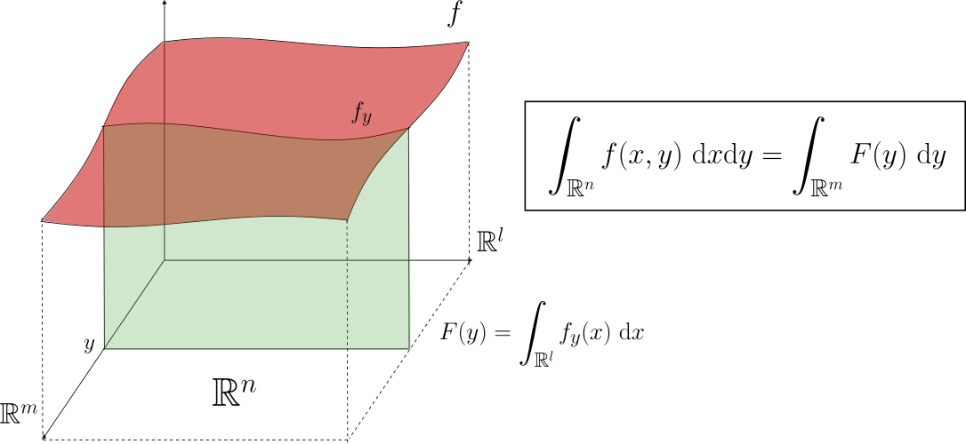
Consideremos una función integrable $f:\mathbb{R}^n\to [-\infty,\infty]$. Como $f$ es medible, es natural pensar que $f_y:\mathbb{R}^l\to [-\infty,\infty]$ «herede cierta regularidad». Supongamos momentáneamente que $f_y$ es integrable para cada $y$ y definamos $$F(y)=\int_{\mathbb{R}^l} f_y(x) \ \mathrm{d}x.$$ Por la misma razón, es esperable pensar que $F$ sea una función integrable.
Intuitivamente, $F(y)$ representa la «masa acumulada» de $f$ en la sección $\mathbb{R}^l\times{ y }$, de modo que la «masa total» de $f$ (i.e. $\int_{\mathbb{R}^n}f(z) \ \mathrm{d}z$) debería ser la «suma» de las contribuciones sobre cada sección. Interpretando a la integral como una «versión continua de la suma», es esperable que:
$$\int_{\mathbb{R}^n}f(z) \ \mathrm{d}z=\int_{\mathbb{R}^m}F(y) \ \mathrm{d}y=\int_{\mathbb{R}^m}\int_{\mathbb{R}^l} f_y(x) \ \mathrm{d}x \ \mathrm{d}y .$$
Esto es precisamente lo que establece el teorema de Fubini.
Por desgracia, es fácil construir ejemplos de funciones medibles $f$, en los que $f_y$ no sea medible para todo $y$.
Ejemplo. Sea $E\subseteq \mathbb{R}^l$ cualquier conjunto no medible y $y_0\in \mathbb{R}^m$ un punto arbitrario. Consideremos $A=E\times{ y_0}\subseteq \mathbb{R}^{l+m}$ y su respectiva función característica $\chi_A$.
Al estar contenido en algún hiperplano, $A$ es un conjunto de medida cero y en automático es medible. En particular $\chi_A$ es una función medible. A pesar de esto, $$f_{y_0}=\chi_{A_{y_0}}=\chi_E.$$ NO es medible sobre $\mathbb{\mathbb{R}}^l$.
$\triangle$
El ejemplo anterior muestra que hay que tener cuidado con la regularidad de las secciones. Afortunadamente, el concepto de casi donde sea nos da una alternativa para resolver este problema como veremos a continuación.
El Teorema de Fubini
Notación. Para enfatizar el hecho de que las integrales debajo son «iteradas», a la integral de una función $f:\mathbb{R}^n=\mathbb{R}^l\times\mathbb{R}^m\to [-\infty,\infty]$, la denotaremos también por $$\int_{\mathbb{R}^n}f(x,y) \ \mathrm{d}x\mathrm{d}y:=\int_{\mathbb{R}^n}f(z) \ \mathrm{d}z.$$ Es decir, solamente reemplazamos $z$ por $(x,y)$ y $\mathrm{d}z$ por $\mathrm{d}x \mathrm{d}y$.
Teorema (Fubini-Tonelli para funciones no negativas). Sea $f:\mathbb{R}^n\to[0,\infty]$ una función medible no negativa. Entonces para c.t.p. $y\in \mathbb{R}^m$, la función $$f_y:\mathbb{R}^l\to [0,\infty]$$ Es medible sobre $\mathbb{R}^l$. Más aún, la función definida en c.t.p. $$F(y)=\int_{\mathbb{R}^l}f_y(x) \ \mathrm{d}x$$ Es medible sobre $\mathbb{R}^m$ y $$\int_{\mathbb{R}^n}f(x,y) \ \mathrm{d}x \mathrm{d}y=\int_{\mathbb{R}^m}F(y) \ \mathrm{d}y=\int_{\mathbb{R}^m}\left( \int_{\mathbb{R}^l}f(x,y) \ \mathrm{d}x\right) \ \mathrm{d}y.$$
La demostración requiere varios pasos, así que la posponemos para futuras entradas. De momento, daremos por hecho el resultado.
Veamos primero un ejemplo sencillo para ver como el teorema de Fubini simplifica en gran medida el cálculo de integrales.
Ejercicio. Calcular la integral $$\int_{(0,\infty)\times(0,\infty)} e^{-(x+y)} \ \mathrm{d}x\mathrm{d}y.$$
Solución. Por definición, queremos calcular, $$\int_{\mathbb{R}^2} e^{-(x+y)}\cdot \chi_{(0,\infty)^2}(x,y) \ \mathrm{d}x\mathrm{d}y.$$
Notemos que podemos escribir $e^{-(x+y)}\cdot \chi_{(0,\infty)^2}(x,y)=e^{-x}\chi_{(0,\infty)}(x)\cdot e^{-y}\chi_{(0,\infty)}(y)$. Ésta es una función medible y no negativa, así que podemos aplicar el teorema de Fubini:
$$\int_{(0,\infty)^2}e^{-(x+y)} \ \mathrm{d}x\mathrm{d}y=\int_{\mathbb{R}}\left( \int_{\mathbb{R}} e^{-x}\chi_{(0,\infty)}(x)\cdot e^{-y}\chi_{(0,\infty)}(y) \ \mathrm{d}x \right) \mathrm{d}y$$
Ahora, en la integral de en medio, el factor $$e^{-y}\chi_{(0,\infty)}(y)$$ NO depende del integrando $x$, así que lo podemos tomar como una constante y «sacarlo de la integral» por linealidad:
$$=\int_{\mathbb{R}} e^{-y}\chi_{(0,\infty)}(y) \left( \int_{\mathbb{R}} e^{-x}\chi_{(0,\infty)}(x) \ \mathrm{d}x \right) \mathrm{d}y$$
$$=\int_{\mathbb{R}} e^{-y}\chi_{(0,\infty)}(y) \left( \int_0^{\infty} e^{-x} \ \mathrm{d}x \right) \mathrm{d}y$$
Ahora el factor $\left( \int_0^{\infty} e^{-x} \ \mathrm{d}x \right)$ NO depende de $y$, por lo que podemos «sacarlo» de la integral por linealidad:
$$=\left( \int_0^{\infty} e^{-x} \ \mathrm{d}x \right)\left( \int_{\mathbb{R}} e^{-y}\chi_{(0,\infty)}(y) \ \mathrm{d}y \right)$$
$$=\left( \int_0^{\infty} e^{-x} \ \mathrm{d}x \right)\left( \int_0^{\infty} e^{-y} \ \mathrm{d}y \right)$$ $$=\left( \int_0^{\infty} e^{-x} \ \mathrm{d}x \right)^2$$
Abreviando el argumento que ya hemos hecho con el teorema fundamental del cálculo y el teorema de la convergencia monótona : $ \int_0^{\infty} e^{-x} \ \mathrm{d}x =\int_0^{\infty} (-e^{-x})’ \ \mathrm{d}x=[-e^{-x}]_{x=0}^{x=\infty}=1$, por lo que: $$\int_{(0,\infty)^2}e^{-(x+y)} \ \mathrm{d}x\mathrm{d}y=1^2=1.$$
$\triangle$
Teorema de Fubini para funciones $L^1$
El teorema de Fubini se puede generalizar fácilmente para funciones en $L^1$.
Teorema (Fubini para funciones $L^1(\mathbb{R}^n)$). Sea $f\in L^1(\mathbb{R}^n)$, Entonces
- $f_y\in L^1(\mathbb{R}^l)$ para c.t.p. $y\in \mathbb{R}^l$. En particular $$F(y)=\int_{\mathbb{R}^l}f_y(x) \ \mathrm{d}x$$ Existe para casi todo $y\in \mathbb{R}^m$.
- $F\in L^1(\mathbb{R}^m)$ y $$\int_{\mathbb{R}^m}F(y) \ \mathrm{d}y=\int_{\mathbb{R}^n}f(x,y) \ \mathrm{d}x\mathrm{d}y.$$
Demostración. Escribamos $f=f_+-f_-$.
Por Fubini-Tonelli se sigue que $f_{\pm,y}$ son funciones medibles en $\mathbb{R}^l$ para casi todo $y\in \mathbb{R}^m$.
$$\implies H(y):=\int_{\mathbb{R}^l}f_{+,y}(x) \ \mathrm{d}x; \ \ \ \ \ \ \ \ \ \ \ G(y):=\int_{\mathbb{R}^l}f_{-,y}(x) \ \mathrm{d}x$$ Existen en c.t.p. $y\in \mathbb{R}^m$. Además de que $$\int_{\mathbb{R}^m}H(y) \ \mathrm{d}y=\int_{\mathbb{R}^n}f_{+}(x,y) \ \mathrm{d}x\mathrm{d}y<\infty$$
Y $$\int_{\mathbb{R}^l}G(y) \ \mathrm{d}y=\int_{\mathbb{R}^n}f_{-}(x,y) \ \mathrm{d}x\mathrm{d}y<\infty.$$
Como las integrales son finitas, se sigue que $H$ y $G$ son finitas para casi todo $y\in \mathbb{R}^m$ (resultado previo). Es decir
$$\int_{\mathbb{R}^l}f_{+,y}(x) \ \mathrm{d}x<\infty;$$ $$\int_{\mathbb{R}^l}f_{-,y}(x) \ \mathrm{d}x<\infty.$$ En c.t.p. $y\in \mathbb{R}^m$. O equivalentemente, que $f_y=f_{+,y}-f_{-,y}\in L^1(\mathbb{R}^l)$ en c.t.p. $y\in \mathbb{R}^m$. Ahora, para tales $y$ tenemos:
\begin{align*}
F(y) &= \int_{\mathbb{R}^l}f_{y}(x) \ \mathrm{d}x \\
&= \int_{\mathbb{R}^l}f_{+,y}(x) \ \mathrm{d}x-\int_{\mathbb{R}^l}f_{-,y}(x) \ \mathrm{d}x \\
&= H(y)-G(x)
\end{align*}
$$\therefore F\in L^1(\mathbb{R}^m)$$ Pues $F$ es igual en c.t.p. a la función $H-G\in L^1(\mathbb{R}^m)$. Además
\begin{align*}
\int_{\mathbb{R}^m}F(y) \ \mathrm{d}y &= \int_{\mathbb{R}^m}H(y) \ \mathrm{d}y-\int_{\mathbb{R}^m}G(y) \ \mathrm{d}y \\
&= \int_{\mathbb{R}^n}f_+(x,y) \ \mathrm{d}x\mathrm{d}y- \int_{\mathbb{R}^n}f_-(x,y) \ \mathrm{d}x\mathrm{d}y \\
&= \int_{\mathbb{R}^n}f(x,y) \ \mathrm{d}x\mathrm{d}y.
\end{align*}
Que es precisamente lo que queríamos probar.
$\square$
Corolario. Supongamos que $f:\mathbb{R}^n\to[-\infty,\infty]$ satisface las hipótesis del Teorema de Fubini (ya sea $f\geq 0$ ó $f\in L^1$). Entonces $$\int_{\mathbb{R}^n}f(x,y) \ \mathrm{d}x\mathrm{d}y=\int_{\mathbb{R}^m}\left( \int_{\mathbb{R}^l}f(x,y) \ \mathrm{d}x \right) \mathrm{d}y=\int_{\mathbb{R}^l}\left( \int_{\mathbb{R}^m}f(x,y) \ \mathrm{d}y \right) \mathrm{d}x.$$
Demostración. La primera igualdad es por supuesto el teorema de Fubini. La segunda igualdad no es más que el resultado de combinar el teorema de Fubini con el cambio de variable
$$(x_1,x_2,\dots,x_l,x_{l+1},\dots,x_n)\to(x_{l+1},\dots,x_n,x_1,x_2,\dots,x_l).$$
$\square$
Integrales iteradas
Mediante varias iteraciones del teorema de Fubini, una integral puede ser descompuesta en integrales iteradas de muchas formas. Por ejemplo, podemos descomponer
\begin{align*}
\int_{\mathbb{R}^n}f(z) \ \mathrm{d}z &= \int_{\mathbb{R}^{n-1}}\left(\int_{\mathbb{R}}f(x,y) \ \mathrm{d}x_1 \right)\mathrm{d}y \\
&= \int_{\mathbb{R}^{n-2}}\left( \int_{\mathbb{R}}\left(\int_{\mathbb{R}}f(x_1,x_2,y’) \ \mathrm{d}x_1 \right) \mathrm{d}x_2 \right) \mathrm{d}y’ \\
&= \dots \\
&= \int_{\mathbb{R}}\left( \int_{\mathbb{R}}\left( \dots \int_{\mathbb{R}} f(x_1,\dots,x_{n-1},x_n)
\ \mathrm{d}x_1 \right)\dots \mathrm{d}x_{n-1} \right) \mathrm{d}x_n
\end{align*}
De igual manera
\begin{align*}
\int_{\mathbb{R}^n}f(z) \ \mathrm{d}z &= \int_{\mathbb{R}}\left(\int_{\mathbb{R}^{n-1}}f(x_1,y) \ \mathrm{d}y \right)\mathrm{d}x_1 \\
&= \int_{\mathbb{R}^m}\left( \int_{\mathbb{R}^l}f(x,y) \ \mathrm{d}x \right) \mathrm{d}y \\
&= \int_{\mathbb{R}}\left( \dots \left( \int_{\mathbb{R}} f(x_1,\dots,x_n)
\ \mathrm{d}x_{\sigma(1)} \right)\dots \right) \mathrm{d}x_{\sigma(n)}
\end{align*}
Son todas descomposiciones válidas. (En este caso $\sigma$ representa una permutación cualquiera de coordenadas).
En general tenemos mucha libertad para descomponer una integral. A la hora de resolver algún problema, es conveniente buscar la descomposición que «nos brinde mayor información» o «mejor se adapte al contexto del problema».
Hasta ahora hemos estado haciendo un gran uso de los paréntesis dentro de las integrales, principalmente para enfatizar el hecho de que las integrales son iteradas. Esto no es del todo necesario y a partir de ahora trataremos de omitirlos para aligerar la notación.
Fubini ayuda a checar integrabilidad
Algo que ocurre con frecuencia es que nos interesa calcular la integral de alguna función $f$ que sólo sabemos que es medible, pero no es $\geq 0$ y no sabemos si pertenece a $L^1$. Es decir, a priori no podemos aplicar el teorema de Fubini.
La manera usual de proceder en estos casos es aplicar el teorema de Fubini a la función $|f|$ (que es no negativa). Con suerte seremos capaces de calcular o estimar: $$\int_{\mathbb{R}
^n}|f(z)| \ \mathrm{d}z=\int_{\mathbb{R}
^m}\int_{\mathbb{R}
^l} |f(x,y)| \ \mathrm{d}x\mathrm{d}y.$$
Para así asegurarnos de que $f\in L^1$ y poder usar Fubini sobre $f$.
Más adelante…
Veremos como el teorema de Fubini se especializa a productos de conjuntos, junto con algunas consecuencias.
Tarea moral
- Calcula $$\int_{\mathbb{R}^2}\frac{1}{(x^2+1)(y^2+1)} \ \mathrm{d}x\mathrm{d}y.$$
- Calcula $$\int_{[0,1]\times [0,\infty)}x e^{-x^2y} \ \mathrm{d}x\mathrm{d}y.$$
- Calcula $$\int_{\mathbb{R}^n} e^{-(x_1+x_2+\dots+x_n)}\mathrm{d}x_1\mathrm{d}x_2\dots \mathrm{d}x_n.$$
- Sean $f:\mathbb{R}^l\to [0,\infty]$ y $g: \mathbb{R}^m\to [0,\infty]$. Supón que la función $h:\mathbb{R}^n\to [0,\infty]$ dada por $h(x,y)=f(x)g(y)$ es medible (de hecho, esto siempre es cierto y es un ejercicio de la siguiente entrada). Demuestra que $$\int_{\mathbb{R}^n}h(x,y) \ \mathrm{d}x\mathrm{d}y=\left( \int_{\mathbb{R}^l} f(x) \ \mathrm{d}x \right) \left( \int_{\mathbb{R}^m} g(y) \ \mathrm{d}y \right).$$ Prueba que lo anterior también es válido si $f\in L^1(\mathbb{R}^l)$ y $g\in L^1(\mathbb{R}^m)$. [SUGERENCIA: Para la segunda parte, aplica primero el teorema de Fubini-Tonelli sobre $|f|$ y $|g|$ para asegurarte de que $h \in L^1(\mathbb{R}^n)$ y poder usar el teorema de Fubini sobre $h$].
- Sea $f:\mathbb{R}^n\to [0,\infty)$ una función no negativa. Supón que la región bajo la gráfica de $f$, $G_f=\{(x,s)\in \mathbb{R}^n\times \mathbb{R} \ | \ 0\leq s \leq f(x)\}$, es un subconjunto medible de $\mathbb{R}^{n+1}$. Sea $g:\mathbb{R}^{n+1}\to [-\infty,\infty]$ una función medible que satisface las hipótesis del teorema de Fubini ($g\geq 0$ ó $g\in L^1(\mathbb{R}^{n+1})$). Demuestra que es posible escribir: $$\int_{G_{f}} g \ \mathrm{d}\lambda=\int_{\mathbb{R}^n}\int_0^{f(x)}g(x,s) \ \mathrm{d}s \mathrm{d}x.$$