(Trabajo de titulación asesorado por la Dra. Diana Avella Alaminos)

INTRODUCCIÓN

Cambiar de base significa que usar otro sistema de referencia para describir a los mismos vectores.

Podemos pensar a la matriz de cambio de base es como una tabla que te indica cómo traducir las coordenadas de un vector de un sistema al otro. Responde entonces al siguiente enunciado: “Si en esta base el vector se ve así, ¿cómo se ve en la otra?”

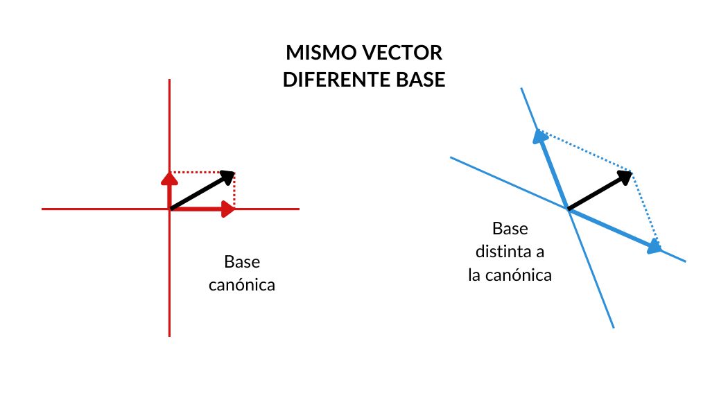
La matriz de cambio de base es la herramienta que nos permite traducir coordenadas de un sistema de referencia a otro, sin cambiar el vector en sí. Es como cambiar de idioma sin cambiar el mensaje.

Es muy útil en matemáticas es tener distintas formas de hacer o representar algo… o mejor dicho, es muy útil saber interpretar, analizar y transformar las diferentes maneras de hacer o representar algo.

MATRIZ DE CAMBIO DE BASE

Definición: Sea $V$ un $K$ – espacio vetorial de dimensión finita $n$. Sean $B$ y $\Gamma$ bases ordenadas de $V$. La matriz de cambio de base de $B$ a $\Gamma$ es $[id_V]_{B}^{\Gamma} \in \mathcal{M}_{n \times n}(K).$

Obs. 1: $[ id_V ]_{B}^{\Gamma}$ es invertible pues $id_V$ es una transformación lineal invertible.

Obs. 2: $\forall v \in V \left( [id_V ]_{B}^{\Gamma}[ v ]_{B}=[id_V(v) ]_{\Gamma} =[ v]_{\Gamma} \right).$

Ejemplos

• Sean $\mathcal{C} = (e_1 , e_2)$ y $\Gamma = ( (2,1) , (-1,2) )$.
  $[id_{\mathbb{R}^2} ]_{\mathcal{C}}^{\Gamma} = \left([ id_{\mathbb{R}^2} ]_{\Gamma}^{\mathcal{C}} \right)^{-1} = \begin{pmatrix} 2 & -1 \\ 1 & 2 \end{pmatrix}.$

Además, si consideramos $T: \mathbb{R}^2 \longrightarrow \mathbb{R}^2$ la reflexión con respecto a la recta $\mathcal{L} = \langle (2,1) \rangle$ se tiene que $T(x,y) = \left( \frac{3x+4y}{5} , \frac{4x-3y}{5} \right)$.

Justificación. Calculemos primero $[id_{\mathbb{R}^2} ]_{\Gamma}^{\mathcal{C}}$ y $[ id_{\mathbb{R}^2} ]_{\mathcal{C}}^{\Gamma}$ por separado. La primera igualdad se cumple por el corolario (3.6.2.) de la entrada 3.6, pero calcular ambas igualdades por separado, nos permite ver la sencillez de calcular $[ id_{\mathbb{R}^2} ]_{\Gamma}^{\mathcal{C}}$ y la dificultad de $[ id_{\mathbb{R}^2} ]_{\mathcal{C}}^{\Gamma}$

Como:
$id_{\mathbb{R}^2} (2,1) = (2,1) = 2e_1 + 1e_2$ y
$id_{\mathbb{R}^2} (-1,2) = (-1,2) = -1e_1 + 2e_2$,
tenemos que:
$[ id_{\mathbb{R}^2} ]_{\Gamma}^{\mathcal{C}} = \begin{pmatrix} 2 & -1 \\ 1 & 2 \end{pmatrix}.$

Para obtener $[ id_{\mathbb{R}^2} ]_{\mathcal{C}}^{\Gamma}$ es necesario resolver un par de sistemas de ecuaciones:

$id_{\mathbb{R}^2} (e_1) = e_1 = \lambda_1 (2,1) + \mu_1 (-1,2) = (2 \lambda_1 – \mu_1 , \lambda_1 + 2 \mu_1)$.
De donde $2 \lambda_1 – \mu_1 = 1$ y $\lambda_1 + 2 \mu_1 = 0$.
Para lo cual $\lambda_1 = \frac{2}{5}$ y $\mu_1 = – \frac{1}{5}$.

$id_{\mathbb{R}^2} (e_2) = e_2 = \lambda_2 (2,1) + \mu_2 (-1,2) = (2 \lambda_2 – \mu_2 , \lambda_2 + 2 \mu_2)$.
De donde $2 \lambda_2 – \mu_2 = 0$ y $\lambda_2 + 2 \mu_2 = 1$.
Para lo cual $\lambda_2 = \frac{1}{5}$ y $\mu_2 = \frac{2}{5}$.

Así, tenemos que:
$[ id_{\mathbb{R}^2}]_{\mathcal{C}}^{\Gamma} = \begin{pmatrix} \frac{2}{5} & \frac{1}{5} \\ – \frac{1}{5} & \frac{2}{5} \end{pmatrix}$

$[ id_{\mathbb{R}^2}]_{\mathcal{C}}^{\Gamma} = \begin{pmatrix} \frac{2}{5} & \frac{1}{5} \\ – \frac{1}{5} & \frac{2}{5} \end{pmatrix}$ $=\frac{1}{5} \begin{pmatrix} 2 & 1 \\ -1 & 2 \end{pmatrix} = \begin{pmatrix} 2 & -1 \\ 1 & 2 \end{pmatrix}^{-1}$ $=\left( [id_{\mathbb{R}^2} ]_{\Gamma}^{\mathcal{C}} \right)^{-1}$.

Concluyendo que $[ (x,y) ]_{\Gamma} = [ id_{\mathbb{R}^2} ]_{\mathcal{C}}^{\Gamma}[(x,y)]_{\mathcal{C}}$ $=\frac{1}{5} \begin{pmatrix} 2 & 1 \\ -1 & 2 \end{pmatrix} \begin{pmatrix} x \\ y \end{pmatrix}$ $=\frac{1}{5} \begin{pmatrix} 2x + y \\ -x+2y \end{pmatrix}$.

Si ahora tomamos $T: \mathbb{R}^2 \longrightarrow \mathbb{R}^2$ la reflexión con respecto a la recta $\mathcal{L} = \langle (2,1) \rangle$.

$T(2,1) = (2,1) = 1(2,1) + 0(-1,2)$
$T(-1,2) = -(-1,2) = 0(2,1) – 1(-1,2)$
$[T ]_{\Gamma}^{\Gamma} = \begin{pmatrix} 1 & 0 \\ 0 & -1 \end{pmatrix}$.

De forma que:
$[ T(x,y) ]_{\Gamma} = [T ]_{\Gamma}^{\Gamma}[ (x,y) ]_{\Gamma}$ $= \begin{pmatrix} 1 & 0 \\ 0 & -1 \end{pmatrix} \frac{1}{5} \begin{pmatrix} 2x+y \\ -x+2y \end{pmatrix}$ $= \frac{1}{5} \begin{pmatrix} 2x+y \\ x-2y \end{pmatrix}$.
$T(x,y) = \frac{2x+y}{5} (2,1) + \frac{x-2y}{5} (-1,2)$ $= \left( \frac{4x+2y}{5} + \frac{-x+2y}{5} , \frac{2x+y}{5} + \frac{2x-4y}{5} \right)$ $= \left( \frac{3x+4y}{5} , \frac{4x-3y}{5} \right)$.

• Sean $V = \{ a+bx | a,b \in \mathbb{R} \}$ y $W = \{ c+dx+ex^2 | c,d,e \in \mathbb{R} \}$
  Sea $T \in \mathcal{L} (V,W)$ tal que $T(3x-4) = 5x^2 + x + 1$ y $T(2x-3) = x^2 – x + 2$.
  $T(a + bx) = (11b + 7a)x^2 + (7b + 5a)x + (-5b-4a).$

Justificación. Sean $\mathcal{C}_1 = (x,1)$, $B = (3x-4 , 2x-3)$ y $\mathcal{C}_2 = (x^2,x ,1)$.

$[ T ]_{B}^{\mathcal{C}_2} = \begin{pmatrix} 5 & 1 \\ 1& -1 \\ 1 & 2 \end{pmatrix}$
$[id_V ]_{B}^{\mathcal{C}_1} = \begin{pmatrix} 3 & 2 \\ -4 & -3 \end{pmatrix}$
$[ id_V]_{\mathcal{C}_1}^{B} = \begin{pmatrix} 3 & 2 \\ -4 & -3 \end{pmatrix}^{-1} = \frac{1}{-1} \begin{pmatrix} -3 & -2 \\ 4 & 3 \end{pmatrix}$

$[ T ]_{\mathcal{C}_1}^{\mathcal{C}_2} =[ T]_{B}^{\mathcal{C}_2}[ id_V ]_{\mathcal{C}_1}^{B}$ $= \begin{pmatrix} 5 & 1 \\ 1 & -1 \\ 1 & 2 \end{pmatrix} \begin{pmatrix} 3 & 2 \\ -4 & -3 \end{pmatrix} = \begin{pmatrix} 11 & 7 \\ 7 & 5 \\ -5 & -4 \end{pmatrix}$

$[ T (a+bx) ]_{\mathcal{C}_2} = [ T ]_{\mathcal{C}_1}^{\mathcal{C}_2} [ a+bx ]_{\mathcal{C}_1}$ $= \begin{pmatrix} 11 & 7 \\ 7 & 5 \\ -5 & -4 \end{pmatrix} \begin{pmatrix} b \\ a \end{pmatrix} = \begin{pmatrix} 11b+7a \\ 7b+5a \\ -5b-4a \end{pmatrix}.$

Así, $T(a+bx) = (11b+7a)x^2 + (7b+5a)x + (-5b-4a)$.

Tarea Moral

1. Sean $B = ( (1,1) , (1,-1) )$ y $\Gamma = ( (2,1) , (-1,1) )$ bases ordenadas de $\mathbb{R}^2.$
   Calcula la matriz de cambio de base de $B$ a $\Gamma$.
   Usa esa matriz para encontrar las coordenadas en $\Gamma$ del vector $v = (3,1)$ sabiendo que $[ v ]_{B} = (2,-1).$
2. Sean $V = P_1[ \mathbb{Q} ]$ y $W = \mathbb{Q}^2.$
   Considera la base ordenada de $V$ $B = ( 1 + x , 1 – x )$ y la base ordenada de $W$ $\Gamma = ( (1,1) , (2,0) ).$
   Sea $T: P_1[ \mathbb{Q} ]\rightarrow \mathbb{Q}^2$ la transformación lineal tal que $T(1+x) = (5 , 2)$ y $T(1-x) = (3 , 2)$. Determina la regla de correspondencia de $T$ indicando cómo es $T(a+bx)$ para toda $a+bx \in P_1[ \mathbb{Q} ].$

Más adelante…

Hasta el momento hemos abordamos la matriz asociada a una transformación lineal cuando tenemos dos bases (una para $V$ y otra para $W$), por otro lado hemos construido la matriz de cambio de coordenadas para cambiar el modo de expresar a un vector, teniendo dos bases distintas para un mismo espacio. Ahora contaremos con una transformación lineal entre dos espacios y cuatro bases (dos para cada espacio vectorial). Así, relacionaremos las matrices asociadas a una misma transformación, con respecto a bases distintas en el dominio y condominio, y observaremos que esta relación está dada por solo una multiplicación de matrices.

Entradas relacionadas

• Ir a Álgebra Lineal I
• Entrada anterior del curso: 3.6. MATRIZ DE UNA COMPOSICIÓN DE TRANSFORMACIONES: invertibles, ejemplos y propiedades
• Siguiente entrada del curso: 3.8. MATRICES CONJUGADAS: matrices de cambio de base