
(Trabajo de titulación asesorado por la Dra. Diana Avella Alaminos)
INTRODUCCIÓN
¿Sabías que cuando compones dos transformaciones lineales puedes predecir exactamente el resultado usando solo sus matrices? Podemos entender cómo es la composición de transformaciones a partir de la multiplicación de matrices. De hecho, si una transformación revierte el efecto de lo que otra hizo (hablamos de una inversa para la transformación), también su matriz puede calcularse a partir de la matriz asociada a la transformación inicial.
Estas ideas abren la puerta a resolver ecuaciones, invertir y comprender procesos con herramientas tan simples como una operación entre matrices.
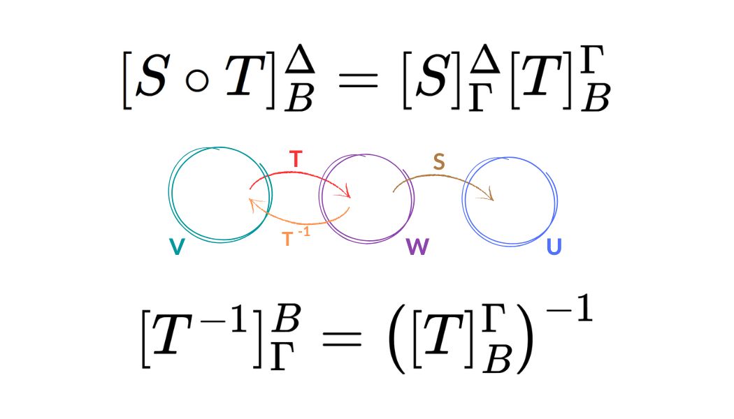
Proposición (3.6.1.): Sean $V,W,U$ $K$-espacios vectoriales de dimensión finita, $B, \Gamma, \Delta$ bases ordenadas de $V$, $W$ y $U$ respectivamente, $T \in \mathcal{L}(V,W)$ y $S \in \mathcal{L}(W,U)$.
Se cumple que: $[ S \circ T ]_{B}^{\Delta} = [ S ]_{\Gamma}^{\Delta} [T ]_{B}^{\Gamma}$
Demostración: Sean $n=\dim V$, $m=\dim W$, $t=\dim U$ y $B = (v_1, …, v_n)$, $\Gamma$ y $\Delta$ bases ordenadas de $V$, $W$ y $U$ respectivamente.
Así, $[S ]_{\Gamma}^{\Delta} \in \mathcal{M}_{t \times m}(K)$ y $[T ]_{B}^{\Gamma} \in \mathcal{M}_{m \times n}(K).$
Por lo tanto, $[S ]_{\Gamma}^{\Delta} [ T ]_{B}^{\Gamma} \in \mathcal{M}_{t \times n}(K)$.
Observamos también que $[S \circ T ]_{B}^{\Delta} \in \mathcal{M}_{t \times n}(K)$. Comparemos entonces las matrices $[ S \circ T ]_{B}^{\Delta}$ y $ [ S ]_{\Gamma}^{\Delta} [T ]_{B}^{\Gamma}$ columna a columna. Sea $j\in\{1,\dots , n\}$.
$col_j [S \circ T ]_{B}^{\Delta}$$=[ S \circ T (v_j) ]_{\Delta}$$=[S(T(v_j)) ]_{\Delta}$$=[ S ]_{\Gamma}^{\Delta}[ T(v_j) ]_{\Gamma}$$=[ S ]_{\Gamma}^{\Delta}[ T ]_{B}^{\Gamma}[ v_j ]_{B}$$=[ S]_{\Gamma}^{\Delta}[ T ]_{B}^{\Gamma} \begin{pmatrix} 0 \\ \vdots \\ 1 \\ \vdots \\ 0 \end{pmatrix}$$=col_j \left( [S ]_{\Gamma}^{\Delta} [T ]_{B}^{\Gamma} \right),$
donde la tercera y cuarta igualdades se justifican con la proposición (3.3.1) de la entrada 3.3.
$\therefore [ S \circ T ]_{B}^{\Delta} = [ S]_{\Gamma}^{\Delta}[ T ]_{B}^{\Gamma}$.
Ejemplos
- Sean $K=\mathbb{R}$, $V=W=\mathbb{R}^2$.
Sea $\mathcal{C}=(e_1,e_2)$ la base canónica ordenada de $\mathbb{R}^2$.
Consideremos $T : \mathbb{R}^2 \longrightarrow \mathbb{R}^2$ la rotación de $\frac{\pi}{2}$ donde $\forall (x,y) \in \mathbb{R}^2 (T(x,y) = (-y,x))$ y $S : \mathbb{R}^2 \longrightarrow \mathbb{R}^2$ la reflexión con respecto al eje $X$ donde $\forall (x,y) \in \mathbb{R}^2 (S(x,y) = (x,-y))$.
Entonces $[ S]_{\mathcal{C}}^{\mathcal{C}} [T ]_{\mathcal{C}}^{\mathcal{C}} = [S \circ T ]_{\mathcal{C}}^{\mathcal{C}}$
Justificación. $S \circ T : \mathbb{R}^2 \longrightarrow \mathbb{R}^2$
$(S \circ T)(x,y)$$= S ( T(x,y) )$$= S (-y,x)$$= (-y,-x)$
$S \circ T (e_1) = (0,-1)$
$S \circ T (e_2) = (-1,0)$
Entonces $[ S \circ T ]_{\mathcal{C}}^{\mathcal{C}} = \begin{pmatrix} 0 & -1 \\ -1 & 0 \end{pmatrix}$.
$T(e_1) = (0,1)$
$T(e_2) = (-1,0)$
Entonces $[T ]_{\mathcal{C}}^{\mathcal{C}} = \begin{pmatrix} 0 & -1 \\ 1 & 0 \end{pmatrix}$.
$S(e_1) = (1,0)$
$S(e_2) = (0,-1)$
Entonces $[ S ]_{\mathcal{C}}^{\mathcal{C}} = \begin{pmatrix} 1 & 0 \\ 0 & -1 \end{pmatrix}$.
$[ S ]_{\mathcal{C}}^{\mathcal{C}} [ T ]_{\mathcal{C}}^{\mathcal{C}}$$=\begin{pmatrix} 1 & 0 \\ 0 & -1 \end{pmatrix} \begin{pmatrix} 0 & -1 \\ 1 & 0 \end{pmatrix}$$=\begin{pmatrix} 0 & -1 \\ -1 & 0 \end{pmatrix}$$=[ S \circ T ]_{\mathcal{C}}^{\mathcal{C}}$.
Corolario (3.6.2.): Sean $V$ y $W$ $K$-espacios vectoriales de dimensión finita con $\dim V=\dim W=n$, $B$ y $ \Gamma$ bases ordenadas de $V$ y $W$ respectivamente y $T \in \mathcal{L}(V,W)$. Se cumple que:
$T$ es invertible si y sólo si $[T ]_{B}^{\Gamma}$ es invertible.
En este caso $[T^{-1} ]_{\Gamma}^{B} = \left([ T ]_B^{\Gamma} \right)^{-1}$.
Demostración: Veamos cada implicación:
$\Rightarrow )$ Supongamos que $T$ es invertible.
Entonces existe $T^{-1} : W \longrightarrow V$ tal que $T^{-1} \circ T = id_V$ y $T \circ T^{-1} = id_W$
Sabemos que $T^{-1} \in \mathcal{L}(W,V)$ y:
1)
$\begin{align*}
[ T^{-1}]_{\Gamma}^{B}[ T ]_{B}^{\Gamma} &= [ T^{-1} \circ T ]_{B}^{B} \tag{Proposición (3.6.1.)}\\
&=[ id_V ]_{B}^{B} \tag{}\\
&= I_n \tag{}\\
\end{align*}$
2)
$\begin{align*}
[ T ]_{B}^{\Gamma}[T^{-1} ]_{\Gamma}^{B} &= [ T \circ T^{-1} ]_{\Gamma}^{\Gamma} \tag{Proposición (3.6.1.)}\\
&=[ id_W ]_{\Gamma}^{\Gamma} \tag{}\\
&= I_n \tag{}\\
\end{align*}$
Así, $[T ]_{B}^{\Gamma}$ tiene inversa y ésta es $[ T^{-1} ]_{\Gamma}^{B}.$
$\Leftarrow )$ Supongamos que $[ T ]_{B}^{\Gamma}$ es invertible, es decir, existe $A\in \mathcal{M}_{n \times n}(K)$ tal que $A [ T]_{B}^{\Gamma} = [T ]_{B}^{\Gamma} A = I_n.$
Por el teorema (3.5.2) de la entrada 3.5 sabemos que $\varphi: \mathcal{L}(W,V) \longrightarrow \mathcal{M}_{n \times n}(K)$ tal que $\forall S\in \mathcal{L}(W,V) \left( \varphi (S) = [ S]_{\Gamma}^{B} \right)$ es un isomorfismo, en particular es suprayectivo y entonces existe $S \in \mathcal{L}(W,V)$ tal que $A = \varphi (S) =[ S ]_{\Gamma}^{B}$
Así, $[ S \circ T ]_{B}^{B} =[ S ]_{\Gamma}^{B} [ T ]_{B}^{\Gamma}=A [ T ]_{B}^{\Gamma}$$=I_n = [ id_V ]_{B}^{B}$
Por el teorema (3.5.2) de la entrada 3.5 sabemos que $\psi : \mathcal{L}(V,V) \longrightarrow \mathcal{M}_{n \times n}(K)$ tal que $\forall S \in \mathcal{L}(V,V)\left( \psi (S) =[ S ]_{B}^{B} \right)$ es un isomorfismo, en particular es inyectivo, de modo que el hecho de que $[ S \circ T ]_{B}^{B} = [ id_V ]_{B}^{B}$ implica que $S \circ T = id_V.$
Análogamente $T \circ S = id_W.$
Así, $T$ tiene inversa y ésta es $S$
$\therefore T$ es invertible.
Ejemplos
- Sean $V = \{ ax + bx^2 + cx^3 | a,b,c \in \mathbb{R} \}$, $W = \{ d + ex + fx^2 | d,e,f \in \mathbb{R} \}$ y $B = (x, x^2, x^3)$, $\Gamma = (1, x, x^2)$ bases ordenadas de $V$y $W$ respectivamente.
Sea $T \in \mathcal{L}(V,W)$ donde $\forall ax + bx^2 + cx^3 \in V \,( T(ax + bx^2 + cx^3) = a+2bx+3cx^2)$.
¿$T$ es invertible? Y si lo es, ¿quién es $T^{-1}$?
Justificación. Es fácil notar que $T^{-1}(d+ex+fx^2)$$=dx+ \frac{e}{2} x^2 + \frac{f}{3}x^3$$\in \mathcal{L}(W,V)$
$T^{-1}(1) = T^{-1}(1+0x+0x^2) = 1x + 0x^2 + 0x^3$
$T^{-1}(x) = T^{-1}(0+1x+0x^2) = 0x + \frac{1}{2} x^2 + 0x^3$
$T^{-1}(x^2) = T^{-1}(0 + 0x + 1x^2) = 0x + 0x^2 + \frac{1}{3} x^3$
$[ T^{-1} ]_{\Gamma}^{B} = \begin{pmatrix} 1 & 0 & 0 \\ 0 & \frac{1}{2} & 0 \\ 0 & 0 & \frac{1}{3} \end{pmatrix}$
$\left( [T]_{\Gamma}^{B} \right)^{-1}$$=\begin{pmatrix} 1 & 0 & 0 \\ 0 & 2 & 0 \\ 0 & 0 & 3 \end{pmatrix}^{-1}$$= \begin{pmatrix} 1 & 0 & 0 \\ 0 & \frac{1}{2} & 0 \\ 0 & 0 & \frac{1}{3} \end{pmatrix}$
$\therefore [ T^{-1} ]_{\Gamma}^{B} = \left( [ T]_{B}^{\Gamma} \right)^{-1}$.
Tarea Moral
- Sea $K = \mathbb{Z}_2.$
Sean $T: K^3 \longrightarrow K^2$ definida para todo $(x,y,z)\in K^3$ como $T(x,y,z) = (x+z , y+z)$ y $S: K^2 \longrightarrow K^4$ definida para todo $(a,b)\in K^2$ como $S(a,b) = (a+b , b , a , 0).$
Considera $B = ( (1,0,0) , (1,1,0) , (1,1,1) )$, $\Delta = ( (1,0) , (1,1) )$ y $\Gamma = ( (1,0,0,0) , (1,1,0,0) , (1,1,1,0) , (1,1,1,1) ),$ bases ordenadas de $K^3,$ $K^2$ y $K^4$ respectivamente.
Calcula $[ S \circ T ]_{B}^{\Delta}.$ - Para cada una de las siguientes transformaciones y bases ordenadas correspondientes, determina si tienen o no inversa y en caso de que sí la tengan calcula $[T^{-1} ]_{\Gamma}^{B}$ y describe la regla de correspondencia de $T^{-1}$:
a) Sea $B = \Gamma= ( (1,0) , (0,1) )$ base de $\mathbb{R}^2$. Sea $T : \mathbb{R}^2 \longrightarrow \mathbb{R}^2$ definida para todo $(x,y) \in \mathbb{R}^2$ como $T(x,y) = (2x+y , x+3y).$
b) Sea $K = \mathbb{Z}_2$, $B = \Gamma= ( (1,0) , (0,1) )$ base de $K^2$. Sea $T: K^2 \longrightarrow K^2$ definida para todo $(x,y) \in K^2$ como $T(x,y) = (x+y , x).$
c) Sea $K = \mathbb{Z}_3$, $B = \Gamma= ( (1,0) , (0,1) )$ base de $K^2$. Sea $T: K^2 \longrightarrow K^2$ definida para todo $(x,y)\in K^2$ como $T(x,y) = (x+y , x+y).$
Más adelante…
Veremos ahora otra matriz especial: La matriz de cambio de base.
Como bien dice su nombre, nos permite pasar de una base a otra.
Cuando leas la definición, medita en por qué la definición de esta matriz refleja precisamente el cambio de un sistema a otro. Al fin y al cabo, recuerda que para cada base podemos representar a cada vector como una combinación lineal de los elementos de la base.
Entradas relacionadas
- Ir a Álgebra Lineal I
- Entrada anterior del curso: 3.5. MATRICES Y TRANSFORMACIONES LINEALES: isomorfismo, ejemplos y propiedades
- Siguiente entrada del curso: 3.7. MATRIZ DE CAMBIO DE BASE: definición y ejemplos