$\textcolor{Red}{\textbf{Funciones de $\mathbb{R}^{n}\rightarrow\mathbb{R}^{m}$ (parte dos)}$

$\textbf{Ejemplo.}$ Encontrar el dominio y la imagen de la región $\displaystyle{R=\left\{(x,y)\in \mathbb{R}^{2}~|~0\leq x\leq1,~0\leq y\leq1\right\}}$ para la función $f:\mathbb{R}^{2}\rightarrow \mathbb{R}^{2}$ dada por $$\displaystyle{f(x,y)=\left(x^{2}-y^{2},2xy\right)}$$

$Solución.$

En este caso $$f_{1}=\left(x^{2}-y^{2}\right)~\Rightarrow~Dom_{f_{1}}=\mathbb{R}^{2}$$
$$f_{2}=\left(2xy\right)~\Rightarrow~Dom_{f_{2}}=\mathbb{R}^{2}$$
por lo tanto
$$Dom_{f}=Dom_{f_{1}}\bigcap Dom_{f_{}}=\mathbb{R}^{2}\bigcap \mathbb{R}^{2}=\mathbb{R}^{2}$$
Para la imagen de la región $\displaystyle{R=\left\{(x,y)\in \mathbb{R}^{2}~|~0\leq x\leq1,~0\leq y\leq1\right\}}$ procedemos de la siguiente manera:
Definimos los siguientes conjuntos que limitan la región

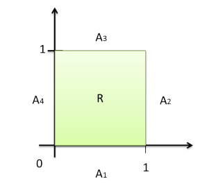
$$A_{1}=\left\{(x,y)\in \mathbb{R}^{2}~|~0\leq x\leq 1,~y=0\right\}$$
$$A_{2}=\left\{(x,y)\in \mathbb{R}^{2}~|~0\leq y\leq 1,~x=1\right\}$$
$$A_{3}=\left\{(x,y)\in \mathbb{R}^{2}~|~0\leq x\leq 1,~y=1\right\}$$
$$A_{1}=\left\{(x,y)\in \mathbb{R}^{2}~|~0\leq y\leq 1,~x=0\right\}$$

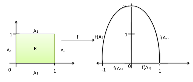
ahora procedemos a encontrar las imagenes de cada uno de los conjuntos definidos

Para $A_{1}$ se tiene
$$A_{1}=\left\{(x,y)\in \mathbb{R}^{2}~|~0\leq x\leq 1,~y=0\right\}f(x,y)=\left(x^{2}-y^{2},2xy\right)=(x’,y’)$$ $$x’=x^{2}-y^{2}~\underbrace{\Rightarrow}_{y=0}~x’=x^{2}~y~si~0\leq x\leq\leq1~\Rightarrow~0\leq x^{2}\leq 1~\Rightarrow~0\leq x’\leq 1$$
$$y’=2xy\underbrace{\Rightarrow}_{y=0}y’=0$$ por lo tanto $$f(A_{1})=\left\{(x’,y’)\in\mathbb{R}^{2}~|~0\leq x’\leq 1~,~y’=0\right\}$$ Para $A_{2}$ se tiene $$A_{2}=\left\{(x,y)\in \mathbb{R}^{2}~|~0\leq y\leq 1,~x=1\right\}f(x,y)=\left(x^{2}-y^{2},2xy\right)=(x’,y’)$$
$$x’=x^{2}-y^{2}~\underbrace{\Rightarrow}_{x=1}~x’=1-y^{2}~\Rightarrow~y=\sqrt{1-x’}$$ $$y’=2xy\underbrace{\Rightarrow}_{x=1}y’=2y~\Rightarrow~y’=2\sqrt{1-x’}~\Rightarrow~y’^{2}=4(1-x’)$$
por lo tanto
$$f(A_{2})=\left\{(x’,y’)\in\mathbb{R}^{2}~|~y’^{2}=4(1-x’),~0\leq y’\leq 2 \right\}$$
Para $A_{3}$ se tiene
$$A_{3}=\left\{(x,y)\in \mathbb{R}^{2}~|~0\leq x\leq 1,~y=1\right\}f(x,y)=\left(x^{2}-y^{2},2xy\right)=(x’,y’)$$
$$x’=x^{2}-y^{2}~\underbrace{\Rightarrow}_{y=1}~x’=x^{2}-1~\Rightarrow~x’+1=x^{2}~\Rightarrow~x=\sqrt{x’+1}$$ $$y’=2xy\underbrace{\Rightarrow}_{y=1}y’=2x~\Rightarrow~y’=2\sqrt{x’+1}~\Rightarrow~y’^{2}=4(x’+1)$$
por lo tanto
$$f(A_{3})=\left\{(x’,y’)\in\mathbb{R}^{2}~|~y’^{2}=4(x’+1),~0\leq y’\leq 2 \right\}$$
Para $A_{4}$ se tiene
$$A_{4}=\left\{(x,y)\in \mathbb{R}^{2}~|~0\leq y\leq 1,~x=0\right\}f(x,y)=\left(x^{2}-y^{2},2xy\right)=(x’,y’)$$
$$x’=x^{2}-y^{2}~\underbrace{\Rightarrow}_{x=0}~x’=-y^{2}ysi0\leq y\leq1~\Rightarrow~0\leq y^{2}\leq 1~\Rightarrow~-1\leq y^{2}\leq 0$$ $$y’=2xy\underbrace{\Rightarrow}_{x=0}y’=0$$
por lo tanto
$$f(A_{4})=\left\{(x’,y’)\in\mathbb{R}^{2}~|~-1\leq x’\leq 0~,~y’=0\right\}$$

$\textcolor{Red}{\textbf{Operaciones con Funciones de $\mathbb{R}^{n}\rightarrow\mathbb{R}^{m}$}}$
$\textbf{Definición 1.}$ Sean $f,g:A\subset \mathbb{R}^{n}\rightarrow\mathbb{R}^{m},\alpha\in\mathbb{R}y~~h:D\subset\mathbb{R}^{m}\rightarrow\mathbb{R}^{k}$. Definimos

1. La suma de f y g que denotamos por f+g como
   $$(f+g)(x)=f(x)+g(x),~~~x\in A$$
2. El producto del escalar $\alpha$ por la función f que denotamos $\alpha f$ como
   $$(\alpha f)(x)=\alpha f(x),~~~x\in A$$
3. El producto punto de f por g que denotamos $f\cdot g$ como
   $$(f\cdot g)(x)=f(x)\cdot g(x),~~~x\in A$$
4. Si $m=3$ el producto cruz de f por g que denotamos $f\times g$ como
   $$(f\times g)(x)=f(x)\times g(x),~~~x\in A$$
5. Si $m=1$ el cociente de f por g que denotamos $\displaystyle{\frac{f}{g}}$ como
   $$\left(\frac{f}{g}\right)(x)=\frac{f(x)}{g(x)},~~~x\in A$$
6. La composición de h con f, que denotamos como $h\circ f$ como
   $$(h\circ f)(x)=h(f(x))para~cada~~\left\{x\in A~|~f(x)\in D\right\}$$

$\textcolor{Red}{\textbf{Gráficas de Funciones de $\mathbb{R}^{n}\rightarrow\mathbb{R}^{m}$}}$

$\textbf{Definición 2.-}$ Dada la función $f (f_{1},…,f_{m}):A\subset\mathbb{R}^{n}\rightarrow
\mathbb{R}^{m}$, definimos su gráfica como el subconjunto
$$g_{f}={(x_{1},…,x_{n},f_{1}(x_{1},…,x_{n}),f_{2}(x_{1},…,x_{n}),…,f_{m}(x_{1},…,x_{n}))\in\mathbb{R}^{n+m}|(x_{1},…,x_{n})\in A}$$

$\textcolor{Red}{\textbf{Límite de Funciones de $f:\mathbb{R}^{n}\rightarrow\mathbb{R}^{m}$}}$

$\textbf{Definición 3. }$$\textcolor{Red}{\textbf{Por sucesiones}}$ Sean $f:A\subset\mathbb{R}^{n}\rightarrow\mathbb{R}^{m}$ y $x_{0}\in A’$. Decimos que f tiene límite en $x_{0}$ y que su límite es $\ell\in\mathbb{R}^{m}$, si para toda sucesión ${x_{k}}$ contenida en $A-{x_{0}}$ que converge a $x_{0}$ se tiene que la sucesión ${f(x_{k})}$ converge a $\ell$. En este caso escribimos
$$\lim_{x\rightarrow x_{0}}f(x)=\ell$$
y decimos que $\ell$ es el límite de f en $x_{0}$.

$\textbf{Definición 4. }$ $\textcolor{Red}{(\epsilon-\delta)}$ Sea $f:A\subset\mathbb{R}^{n} \rightarrow
\mathbb{R}^{m}$, y sea $x_{0}$ un punto de acumulación de A.
Se dice que $\ell\in\mathbb{R}^{m}$ es el límite de $f$ en
$x_{0}$, y se denota por:\ $$\displaystyle\lim_{x\rightarrow
x_{0}}f(x)=\ell$$ Si dado $\forall~\epsilon > 0$, existe $\delta > 0$ tal
que $$|f(x)-\ell|<\epsilon~cuando~0<|x-x_{0}|<\delta$$

$\textcolor{Red}{\textbf{Continuidad de Funciones de Varias Variables}}$

$\textbf{Definición 5.}$ Sean $f:\Omega\subset\mathbb{R}^n\rightarrow\mathbb{R}^m$ y
$x_0\in\Omega$. Se dice que $f$ es continua en $x_0$ si dado $\epsilon>0$, $\exists$ $\delta>0$ tal que $|f(x)-f(x_0)|<\epsilon$ siempre que $x\in\Omega$ y $0<|x-x_0|<\delta$

$\textbf{Definición 6.}$ Se dice que un subconjunto $V\subset\mathbb{R}^{n}$ es un entorno del punto $x$, si exite $\epsilon>0$ tal que $B(x,\epsilon)\subset V.$

$\textbf{Definición 7.}$ Sean $f:\Omega\subset\mathbb{R}^n\rightarrow\mathbb{R}^m$ y $x_0\in\Omega$. Se dice que $f$ es continua en $x_0$ cuando $\forall$ entorno V de $f(x_{0})$ existe un entorno U de $x_{0}$ tal que $f(U)\subset V$ es decir para cualquier $x\in U$ se cunple $f(x)\in V$

$\textbf{Proposición 1.}$

Una función $f:D\subset\mathbb{R}^{n}\rightarrow \mathbb{R}^m$ es continua si y solo si
$$f^{-1}(v)=\left\{x\in D\mid f(x)\in v\right\}$$
es un abierto (contenido en $D$) para cada abierto $v\subset\mathbb{R}^m$.

$Demostración$

$\textcolor{Red}{\Rightarrow}$ Sea $v$ un abierto en $\mathbb{R}^m$ y sea $\overline{x}\in f^{-1}(v)$; tenemos por definición $f(\overline{x})\in v$. Como $v$ es un
conjunto abierto $\exists\ \ r>0$ tal que $B(f(\overline{x}),r)\subset v$ como $f$ es continua $\exists$ $\rho>0$ tal que $f(B(x,\rho))\subset B(f(x),r)$ pero esto significa que $B(x,\rho)\subset f^{-1}(B(f(x),r))\subset f^{-1}(v)$ por lo que cada punto $x\in f^{-1}(v)$ es punto interior lo que prueba que $v$ es abierto.
$\textcolor{Red}{\Leftarrow}$ Supongamos que $f^{-1}(v)$ es un abierto, para cada conjunto abierto $v\subset\mathbb{R}^{m}$\Sea $\epsilon>0$ y $x\in\mathbb{R}^{n}$, hacemos:
$B(f(x),\epsilon)=V$ por lo que$f^{-1}(V)$ es abierto, esto quiere decir que $\exists~\delta>0$ tal que $B(x,\delta)\subset f^{-1}(V)$ esto implica $f(B(x,\delta))\subset V$ esto es $f(B(x,\delta))\subset B(f(x),\epsilon)$ esto muestra que $f$ es continua en $x$.

$\textbf{Proposición 2.}$

(1) $$f^{-1}(v)=\left\{x\in D\mid f(x)\in v\right\}$$
es un abierto (contenido en $D$) para cada abierto
$v\subset\mathbb{R}^m$.
(2) $$f^{-1}(v)=\left\{x\in D\mid f(x)\in v\right\}$$
es un cerradoo (contenido en $D$) para cada cerradoo
$v\subset\mathbb{R}^m$.

Vamos a probar que $\textcolor{Red}{1\Rightarrow 2}$

$Demostración$

Si $V=\overline{V}\subset\mathbb{R}^{m}$, consideremos el conjunto $V^{c}$ el cual es abierto y por hipotesis $f^{-1}(V^{c})$ es abierto, pero
$$f^{-1}(V^{c})=\left(f^{-1}(V)\right)^{c}$$
por lo que $\left(f^{-1}(V)\right)^{c}$ es abierto, en consecuencia $f^{-1}(V)$ es cerrado\
Vamos a probar que \textcolor{Red}{$2\Rightarrow 1$}
Si $V=int(V)\subset\mathbb{R}^{m}$ entonces $V^{c}$ es cerrado y por hipotesis $f^{-1}(V^{c})$ es cerrado, pero
$$f^{-1}(V^{c})=\left(f^{-1}(V)\right)^{c}$$
por lo que $\left(f^{-1}(V)\right)^{c}$ es cerradoo, en consecuencia $f^{-1}(V)$ es abierto $\square$