En éste apartado se abordará otra metodología para valuar proyectos de inversión la cual es conocida como Valor presente neto, que como su nombre lo indica, consiste en determinar el valor presente de los flujos.
Método del Valor Presente Neto
Consiste en obtener el valor presente de los flujos de efectivo netos, con una cierta tasa esperada de rendimiento. Dicha tasa, queda determinada o pactada por el inversionista, en base a sus aspiraciones que tenga sobre el negocio, Para ello pueden hacer uso de tasas de referencia como el CETE, la TIIE, etc.
Procedimiento
Determinar el flujo neto así como, calcular los flujos de ingreso y de egresos.
Obtener el valor presente de todos los flujos netos usando la tasa de rendimiento esperada.
Realizar la suma de todos los valores presentes para obtener el Valor Presente Neto del proyecto de inversión.
Criterio:
Si el Valor Presente Neto es igual o mayo a cero, entonces aprueban el proyecto
Si el Valor Presente Neto es negativo, es decir; menor que cero, entonces se rechaza el proyecto.
$i=$ tasa de rendimiento a la que se descuentan los flujos
$v=\frac{1}{(1+i)}$
$d=$ tasa de descuento equivalente a $i$
$n=$ número de años del proyecto
Reglas para su aplicación:
Hay proyectos de inversión, en los que la fecha de inicio es a fin de año, lo cual puede ocasionar que la ecuación del modelo que estamos usando, comience en la potencia cero, es decir: $v^0$
Cuando se tengan proyectos donde los flujos terminen en el año $n$, se considera que dicho plazo corresponde a la vida útil del proyecto. Sin embargo, los proyectos puede ocurrir que los proyectos continúen por más años.
Para los casos en los que ocurre que los proyectos continúan existiendo por más tiempo, para calcular el VPN total, se determinan los ingresos y egresos para los años siguientes (regularmente se establece un flujo fijo), es decir; se obtiene su calor presente y se le suma al VPN calculado en la primer instancia.
$$VPNT=\sum F_jv^n+\sum F_kv^{m+n}$$
lo anterior, con flujos de efectivo para cada año después del $n$
$$VPNT=\sum F_jv^n+\sum \frac{Fc}{i}v^{n}$$
la expresión anterior, con flujos iguales para cada año, después del $n$
Cabe hacer mención que hay una variante del método del VPN, el cual se llama Valor Presente Ajustado (VPA), el cual se obtiene restando al VPN el costo de oportunidad al capital que se invirtió.
$VPA=VPN-$ costo de oportunidad
El costo de oportunidad, se entenderá como «la pérdida o costo» que se incurre al haber seleccionado la opción «X» en lugar de la opción «Y». Dicho costo de oportunidad se calcula valuando los flujos de efectivo, que se obtendrían de haber invertido los recursos en un instrumento bancario de renta fija.
Ejercicios resueltos
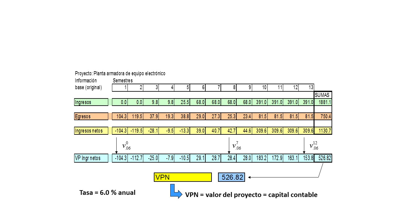
Ejercicio. En el siguiente ejercicio tenemos el siguiente planteamiento: Un inversionista destino sus recursos al siguiente proyecto de inversión en una empresa que se dedica a armar equipo electrónico, de la cual obtuvo los siguientes registros y desea calcular el Valor Presente Neto de dicho proyecto.
Solución
Para hacer el cálculo del VPN se tuvieron que hacer uso de la siguiente información
En dicho ejercicio se observa que se trae a valor presente cada uno de los flujos, de cada periodo. Luego se realiza la suma del resultado de obtenido en cada valor presente, lo que como se había comentado, es el valor presente neto del proyecto de inversión
Ejercicio. A continuación se muestran flujos de efectivo de un proyecto de inversión,De acuerdo a la siguiente lista:
0. -1000, en el periodo
se registra una cantidad de 100,
se registra una cantidad de 200
se registra una cantidad de 700
se registra una cantidad de 700
Y el inversionista quiere saber, por medio del método del Valor Presente Neto, si dicho proyecto le conviene
Como el Valor Presente Neto (VPN)>0, entonces el proyecto es aceptado
Más adelante…
A lo largo de este material se continuara abordando otros métodos para valuar proyectos de inversión, con la finalidad de evidenciar su importancia, así como la forma en que deben de utilizarse en la práctica real.
En éste apartado, se abordará un tema importante dentro de las Matemáticas Financieras, ya que nos provee de un panorama general, sobre como podemos hacer uso de éstas, para poder aplicar los conocimientos adquiridos; en el sentido de que se mostrará como realizar análisis de proyecto de inversión. Se partirá realizando una descripción de lo que se entiende como proyecto de inversión, estableciendo sus características, así como sus alcances, las variables que intervienen, así como, algunos modelos que podemos usar y sus reglas para su aplicación.
Definición de proyecto de inversión
Un proyecto, es un modelo sistemático que define y engloba un conjunto de acciones, así como la forma en que se deben de llevar a cabo para alcanzar determinadas metas u objetivos. En dicho modelo se establecerán la forma, los recursos necesarios que se vayan a utilizar, para poder llevarlo a cabo de manera satisfactoria.
La palabra inversión, es un término que se utiliza para definir ahorro, o colocar recursos económicos que se ponen en un lugar determinado, con el fin de obtener algún beneficio que incremente la cantidad inicial después de cierto tiempo, como por ejemplo aumentar una cantidad de dinero, ganando intereses. En términos de dinero, sería gastarlo o utilizarlo de otra manera.
Por lo anterior, se entenderá como proyecto de inversión como el conjunto de elementos o variables necesarias para alcanzar una meta o un fin de índole económica, el cual consiste en esencia, en manejar, utilizar, o una cierta cantidad de recursos financieros, de una forma diferente a la que usualmente se viene realizando, para poder obtener un mejor beneficio de recursos económicos.
Es pertinente señalar que la definición antes mencionada, implica que se debe de tener al menos una diferente opción a la que se viene manejando. Dicha opción debe de contar con ciertas características, en términos de dinero destacan: productividad, rendimiento, e interés.
El objetivo que tiene la evaluación de proyectos de inversión, es el de establecer y determinar si dichas opciones que se tienen para invertir los recursos económicos, es mejor, igual o peor que la que actualmente se tiene.
Características de los proyectos de inversión
Partiendo de la definición de proyecto de inversión, se puede identificar que hay inversiones de índole puramente financiera que tienen la finalidad de obtener una ganancia o utilidad mayor. También existen proyectos de inversión que tiene que ver con algún tipo de obra, ya sea de tipo arquitectónico, físico, adquisición de programas de cómputo, patentes, adquisición de maquinaria, adquisición de una empresa o parte de ella, etc.
Ambos casos se pueden valuar, y se puede apreciar que las dos tienen como objetivo principal, un beneficio económico, un tipo de recompensa. En la mayoría de los casos, dichas valuaciones se pueden llevar a cabo mediante, la comparación de una tasa de interés emitida por una banco X, con respecto a la que emite un banco Y.
Con respecto segundo caso de la valuación de proyectos de inversión que tienen que ver con obras o adquisición de empresas, etc. dicha valuación, es más complicada de llevar a cabo, ya que involucra aspectos más complejos porque tiene que ver con tiempos más largos, dentro de los cuales, hay flujos de recursos de entrada y salida. Para éstos tipos de casos es que se han desarrollado varias metodologías.
Objetivos de los proyectos de inversión
El objetivo principal de los proyectos de inversión es el de poder determinar la tasa de rentabilidad que ofrece un proyecto de inversión, para que con ésa información se pueda tomar mejores decisiones, como por ejemplo: tener el conocimiento para invertir en la opción que ofrezca el mayor rendimiento, no invertir en proyectos que no tengan rentabilidad o sea mínima, o bien poder determinar los aspectos que afectan o favorecen dicha rentabilidad.
La valuación de proyectos de inversión nos permite también, poder conocer en qué tiempo vamos a poder recuperar la inversión que se haya realizado.
Es pertinente hacer mención que dentro de éste apartado se abordarán las metodologías que para valuar proyectos de inversión en los que no se tiene considerada de forma explícita variables de riesgo.
Algunos ejemplo en los que se tiene garantía para recuperar la inversión realizada serían:
Los depósitos bancarios a cierto plazo, como los siguientes:
El banco «Mi ahorro», ofrece una tasa de interés del 5.4% anual, y el banco «Le money» ofrece una tasa del 7.8% anual. En éste caso se selecciona al banco «Le money» como la mejor opción para hacer la inversión.
El banco «X» ofrece una tasa de rendimiento del 1.1715% efectiva mensual. Así mismo, el banco «Y» ofrece una tasa de interés del 15% efectiva anual. Para poder determinar cuál es la opción en la que más conviene hacer la inversión, lo que se tiene que hacer es calcular la tasa equivalente del 15% efectiva anual, con respecto a la tasa del 1.1715% pagadera diaria. En este caso tenemos que al efectuar el cálculo para obtener la tasa equivalente, llegamos a la conclusión de que es la misma tasa, por lo que, cualquiera de los dos bancos es viable para hacer la inversión.
Ejercicios resueltos
Ejercicio. El banco Alfa, ofrece una tasa de interés del 7.4% pagadero diario, mientras que el banco Beta, ofrece una tasa de interés del 7.4% efectivo anual. ¿Qué opción es la que mas conviene invertir?
Solución
Para obtener la respuesta a éste ejercicio, lo que se tiene que realizar es calcular la tasa equivalente efectiva anual de la tasa 7.4% pagadero diario, con la finalidad de poder compararla con la tasa efectiva anual del 7.4%
Usando la triple igualdad se tiene que la tasa equivalente es del 7.6% efectiva anual.
Por lo tanto, la opción que le conviene más invertir es la que ofrece el banco «Alfa».
Más adelante…
En el siguiente apartado se continuarán revisando más metodologías para valuar proyectos de inversión, específicamente la TIR, se definirán sus características, sus reglas de aplicación y se establecerá la relación que hay entre costo y beneficio.
En este apartado, se aborda el tema de funciones y factores de acumulación, donde se darán a conocer sus características o propiedades, su forma en que operan y algunos ejemplos de su aplicación. El factor de acumulación, es la manera a través de la cual los intereses se van creciendo, ya sea de forma lineal como lo es en el modelo de interés simple, o de forma compuesta, es decir; los intereses generan intereses, por lo que el crecimiento de éstos recursos es más rápido. Se entiende como valor acumulado como la cantidad total que se obtiene luego de que haya transcurrido un cierto periodo de tiempo.
Función de acumulación
Es aquella función que acumula una unidad monetaria, iniciando en un tiempo cero, luego de haber transcurrido un tiempo $t$, todo ésto con una tasa de interés. Tanto la tasa de interés como el periodo de tiempo, deben estar dados con la misma periodicidad, es decir, si por ejemplo: si el tiempo es anual, la tasa de interés que se esté manejando, igual debe de ser anual.
Cabe hacer mención, que hay función de acumulación para el modelo de interés simple, y hay función de acumulación para el modelo de interés compuesto.
Función de acumulación para interés simple
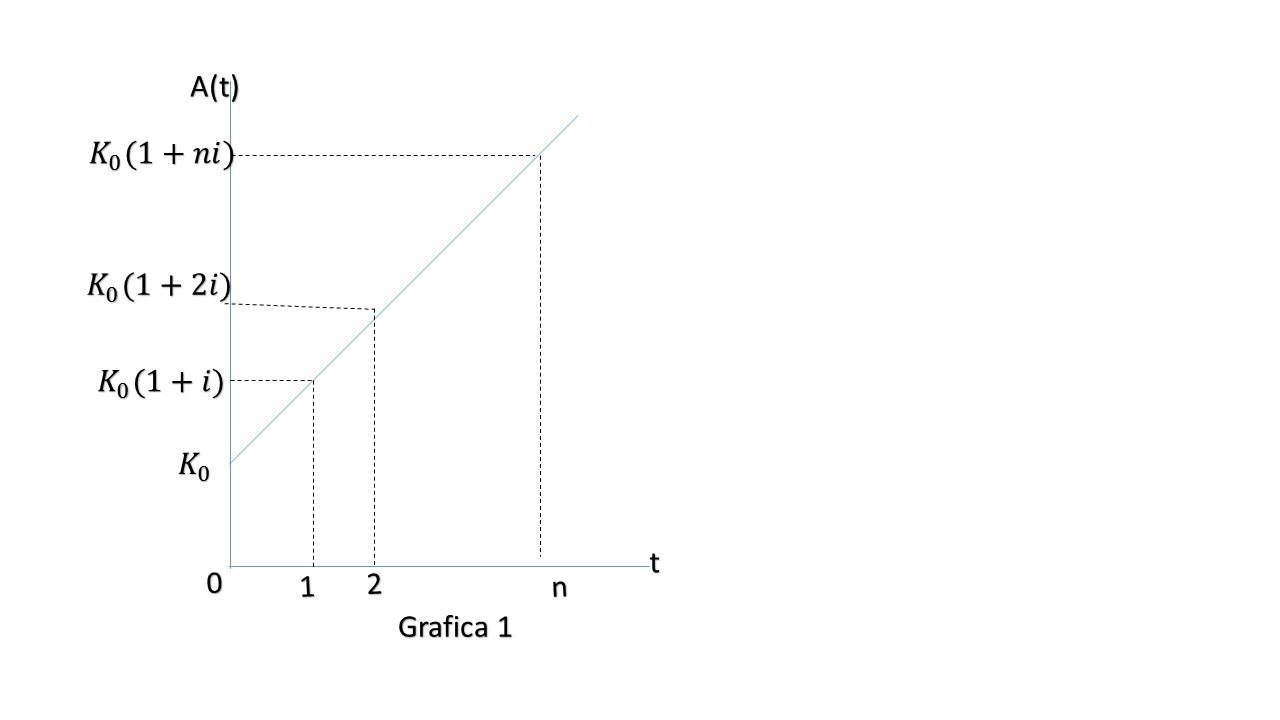
La acumulación simple que se utiliza en éste modelo, es aquella en la que el crecimiento de los intereses, se da de forma lineal, es decir, los intereses que se generan en un mismo periodo de tiempo, no se acumulan (no generan nuevos intereses) en el siguiente periodo. Dicha acumulación se puede calcular en cualquier momento.
La función de acumulación en este modelo de interés simple, es la función que se define como $a(t)$ que lleva un valor acumulado, luego de transcurrir un tiempo $t>0$. En este caso el capital que se va a manejar es de una unidad monetaria. Dicha función de acumulación $a(t)$ cumple que:
Es creciente y continua regularmente
En un valor $a(0)=1$
Si la función de acumulación va disminuyendo, para valor de $a$ con valores de $t$ crecientes, esto implica que hay un interés negativo.
Aunque puede ocurrir que haya intereses negativo, para efectos prácticos es irrelevante, para la mayoría de la situaciones.
El capital inicial que se invierte se le llama $K$ y es una cantidad mayor que cero, es decir; $K>0$.
$A(t)$ es la función monto con la que se obtiene el valor acumulado en el tiempo $t>0$ con un capital determinado $K$
Lo que se acaba de mencionar se traduce en lo siguiente:
$$A(t)=K a(t)$$
$$A(0)=K$$
Se denota la cantidad de intereses ganado durante un periodo de tiempo $t-$ésimo año, en una fecha de inversión $I_t$. Es decir:
$$I_t =A(t)-A(t-1)$$
para $t\leq 1$. Observe que $I_t$ considera el efecto del interés sobre un periodo $t$, en cambio $A(t)$ es una cantidad que se calcula en un tiempo determinado.
La función monto de acumulación que se tiene, cuando se está trabajando con un capital de un peso, es decir $K=1$, es una caso especial de dicha función de acumulación. En ambos casos, tanto la función de acumulación como la función monto se pueden usar de forma recíproca.
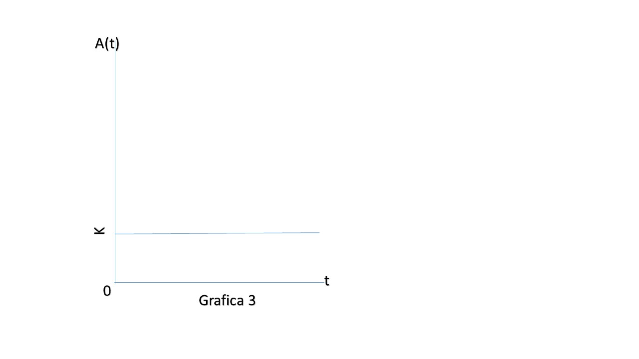
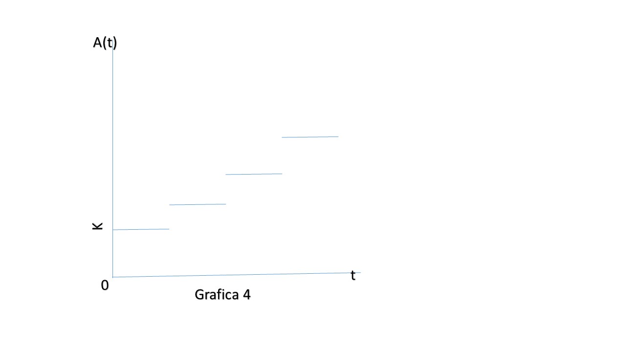
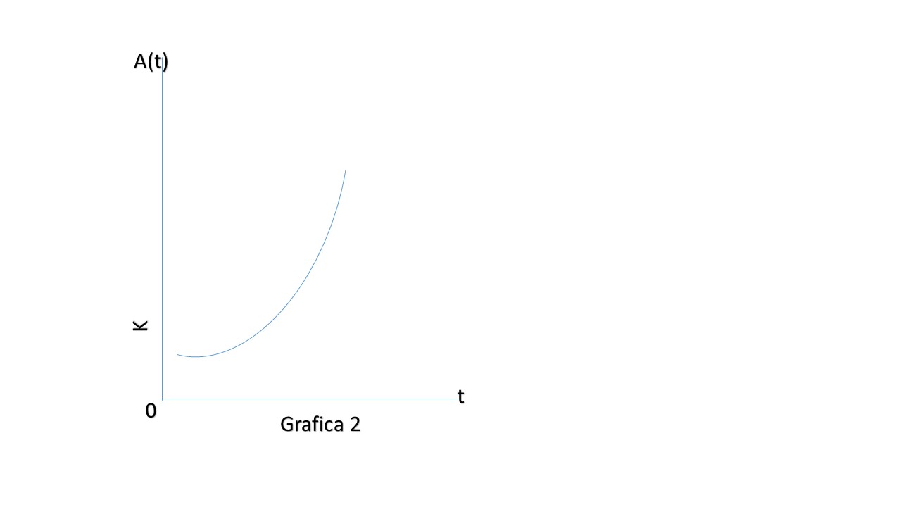
A continuación se muestran ejemplo del comportamiento de la función monto.
Elaboración propia. Comportamiento de la función de acumulación con el modelo de interés simpleElaboración propia. Comportamiento de la función de acumulación con el modelo de interés simple, pero es una gráfica que nos dice que no genera intereses.Elaboración propia. Comportamiento de la función de acumulación con el modelo de interés simple, pero es una gráfica que nos dice que no está acumulando de forma continua, puede darse cuando el interés se paga al final del periodo.
Función de acumulación para el modelo de interés compuesto
En este modelo, la función de acumulación lo intereses del capital inicial, generan intereses sobre intereses, es decir; los intereses se reinvierten ganando más intereses, por dicha característica se le conoce a este fenómeno como acumulación compuesta.
La función de acumulación, se define como la que acumula una unidad monetaria comprendido desde un momento cero, hasta un tiempo $t$ con una acumulación compuesta, y con una tasa efectiva de interés $i$, que debe coincidir con la temporalidad del tiempo, y viceversa. Dicha función es denotada por:
$$A(t)=(1+i)^t$$
Desarrollando dicha expresión de en la que está dada se comporta de la siguiente forma:
$$A(1)=1+i$$
$$A(2)=(1+i)(1+i)=(1+i)^2$$
$$A(3)=(1+i)(1+i)(1+i)=(1+i)^3$$
$$\vdots$$
$$A(t)=(1+i)^t$$
Elaboración propia. Comportamiento de la función de acumulación con el modelo de interés compuesto
La función de acumulación es válida para toda $t$. Es importante hacer mención ya que $t$ pertenece a intervalo $t \in[0,\infty)$, se puede ampliar a $A(t)$ para comprobar que la función es válida para dicho intervalo.
Entonces, sea $t \geq 0$, y $s \geq 0$
Partiendo de $(1+i)^t$ se tiene que:
$$A(t+s)=(1+i)^{t+s}$$
$$=(1+i)^t (1+i)^s=(A(t))(A(s))$$
a dicha expresión se le aplica la definición de derivada y entonces se obtiene:
Sustituyendo éste ultimo resultado, en $ln A(t)- ln A(0)=tA'(0)$, se da lugar a:
$$ln A(t)=t ln(1+i)=ln(1+i)^t$$
$$A(t)=(1+i)^t \forall t\geq 0$$
dicha expresión que se acaba de obtener, se puede escribir de la siguiente forma:
$$A(t)=A(0)(1+i)^t$$
Más adelante…
En las siguientes apartados se mostrara que diferentes maneras de como se pueden dar este proceso de acumulación, para fines de aplicación en la práctica real, sólo es necesario que se haga uso de 2 funciones de acumulación, que corresponde al modelo de interés simple y de interés compuesto.
El contenido de esta sección se basa predominantemente en el libro Wheeden, R.L., Zygmund, A., Measure and Integral. An Introduccion to Real Analysis. (2da ed.). New York: Marcel Dekker, 2015, págs 17-22.
Estamos por presentar las últimas notas de blog del curso de Análisis Matemático I. Pretendemos mostrar un puente entre lo que vimos aquí y lo que se aprenderá en Análisis Matemático II. Conoceremos algunas ideas que, eventualmente, nos llevarán al concepto de la integral de Riemann-Stieltjes, un concepto que generaliza a la integral de Riemann (que suele verse en los cursos de Cálculo) pero que también es un caso particular de la integral de Lebesgue, la que se verá en la siguiente sección del blog. Para comenzar, analicemos los cambios que una función va tomando en un dominio cerrado.
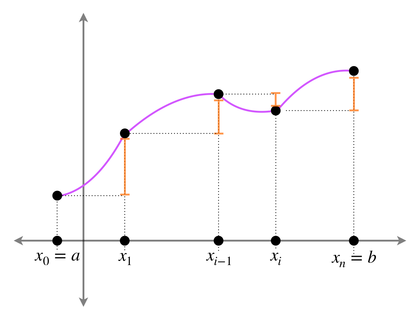
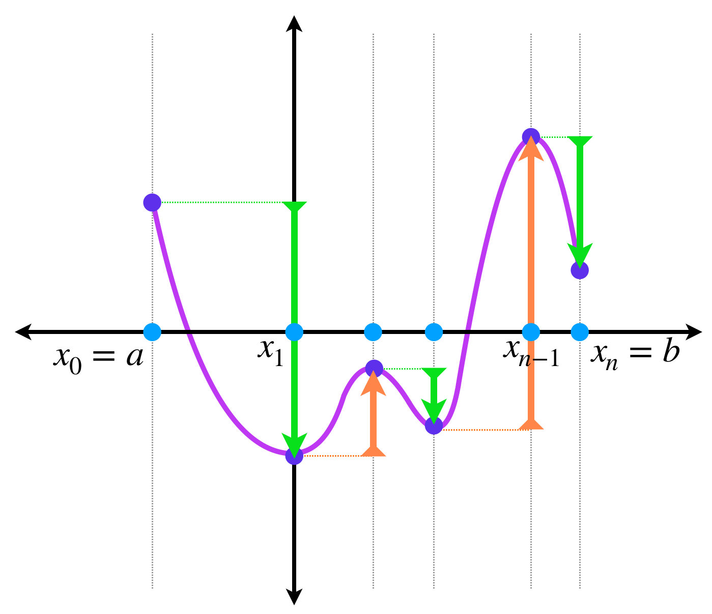
Definición. Partición de un intervalo $\textbf{[a,b].}$ Sea $[a,b]$ un intervalo de $\mathbb{R}.$ Si $P = \{x_0=a, \, x_1, \, x_2,…,x_{n-1}, \, x_n = b\}, \, i=0,1,2,…,n \,$ es una colección de puntos tales que $x_0 =a, \, x_n = b$ y para cada $i =1,2,…,n$ se cumple que $x_{i-1}< x_i,$ entonces diremos que $P$ es una partición de $[a,b].$
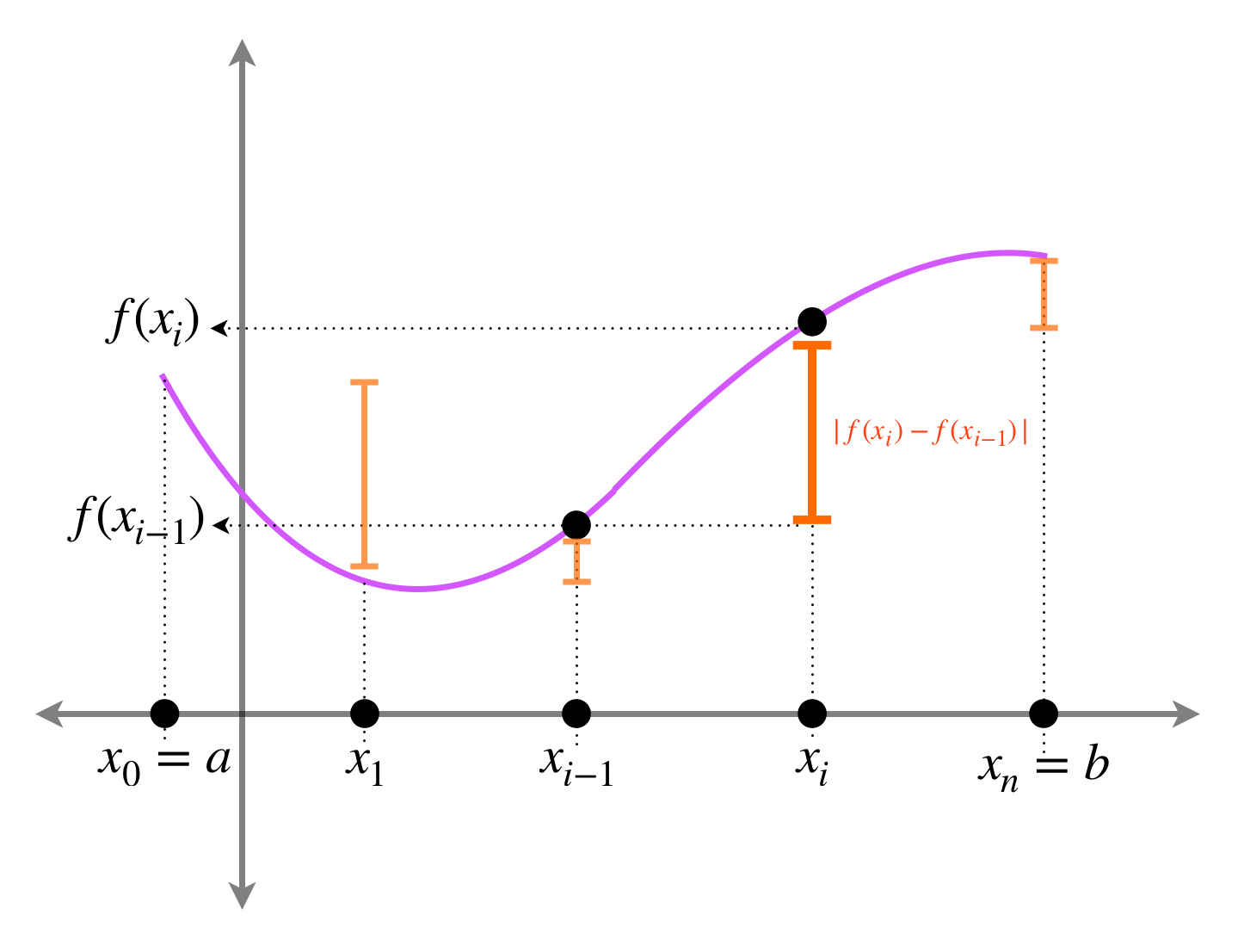
Definición. Variación de $f$ sobre $[a,b].$ Considera una función $f:[a,b] \subset \mathbb{R} \to \mathbb{R} \,$ y sea $P=\{x_0, \, x_1, \, …, \, , x_n\}$ una partición de $[a,b].$ Definimos $S_P[f;a,b]$ (o bien $S_P$ cuando no hay necesidad de especificar la función y el intervalo) como: $$S_P[f;a,b] := \sum_{i=1}^{n}|f(x_i) \, -\, f(x_{i-1})|$$
La suma del tamaño de los segmentos naranjas es la $S_P.$
Entonces se suman las distancias que se generan al evaluar $f$ en cualesquiera dos puntos consecutivos de la partición.
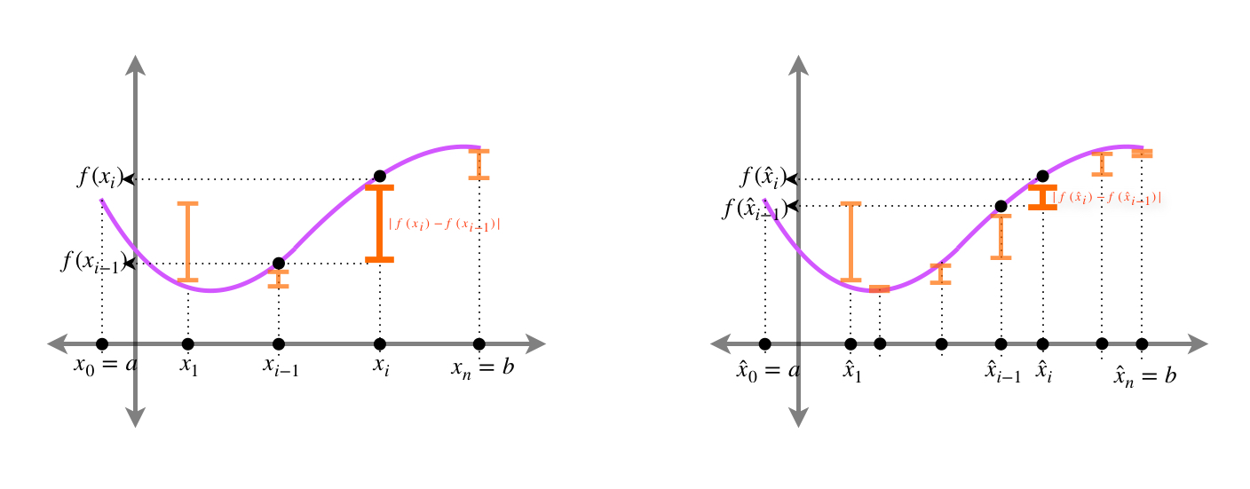
Ya que para cada partición $P$ de $[a,b]$ existe su respectiva $S_P,$ podemos pensar en si la colección de todas las sumas tiene supremo. El supremo de las sumas de todas las particiones de $[a,b]$ recibe el nombre de variación de $f$ sobre $[a,b].$ Se denota como: $$ \underset{P \, \in \, \mathcal{P_{[a,b]}}}{sup} \, S_P \, :=V[f;a,b] \, := V [a,b]\, := V$$
Donde $\mathcal{P}_{[a,b]} \,$ es el conjunto de particiones de $[a,b].$
Las sumas pueden dar resultados distintos con particiones distintas.
Definición. Función de variación acotada y de variación no acotada. Sea $f:[a,b] \to \mathbb{R}.$ Considera $V[f;a,b].$ Si el supremo de hecho existe en $\mathbb{R},$ entonces $0 \leq V$ y diremos que $f$ es de variación acotada en $[a,b].$ En otro caso diremos que $V = \infty \,$ y que $f$ es de variación no acotada.
Ejemplos de variación en funciones
A continuación presentamos las variaciones de algunas funciones. Al final de esta sección te pediremos calcular los resultados formalmente.
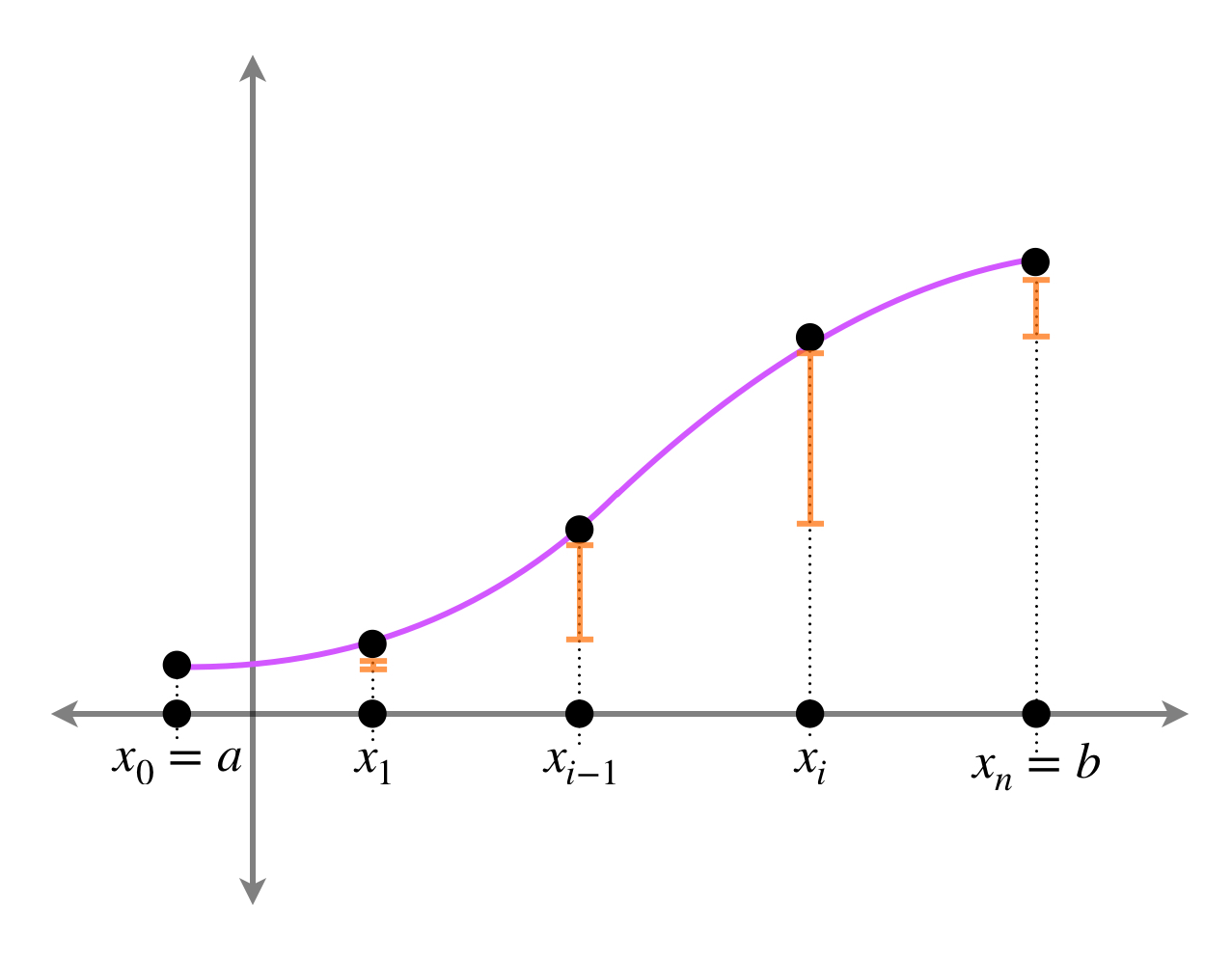
Sea $f:[a,b] \to \mathbb{R} \,$ tal que $f$ es monótona. Entonces para cualquier partición $P,$ $$S_P=|f(b) \, – \, f(a)|=V.$$
Si $f$ es monótona la suma de los segmentos naranjas es $|f(b) \, – \, f(a)|.$
Sea $f:[a,b] \to \mathbb{R}$ tal que $f$ puede expresarse en pedazos monótonos acotados, es decir, existe una partición $P = \{x_0 =a, \, x_1,…,x_n =b\}$ tal que $f$ es monótona en cada intervalo $[x_{i-1}, \, x_i].$ Entonces $$V = S_P.$$
$f$ es monótona en cada intervalo $[x_{i-1}, \, x_i].$
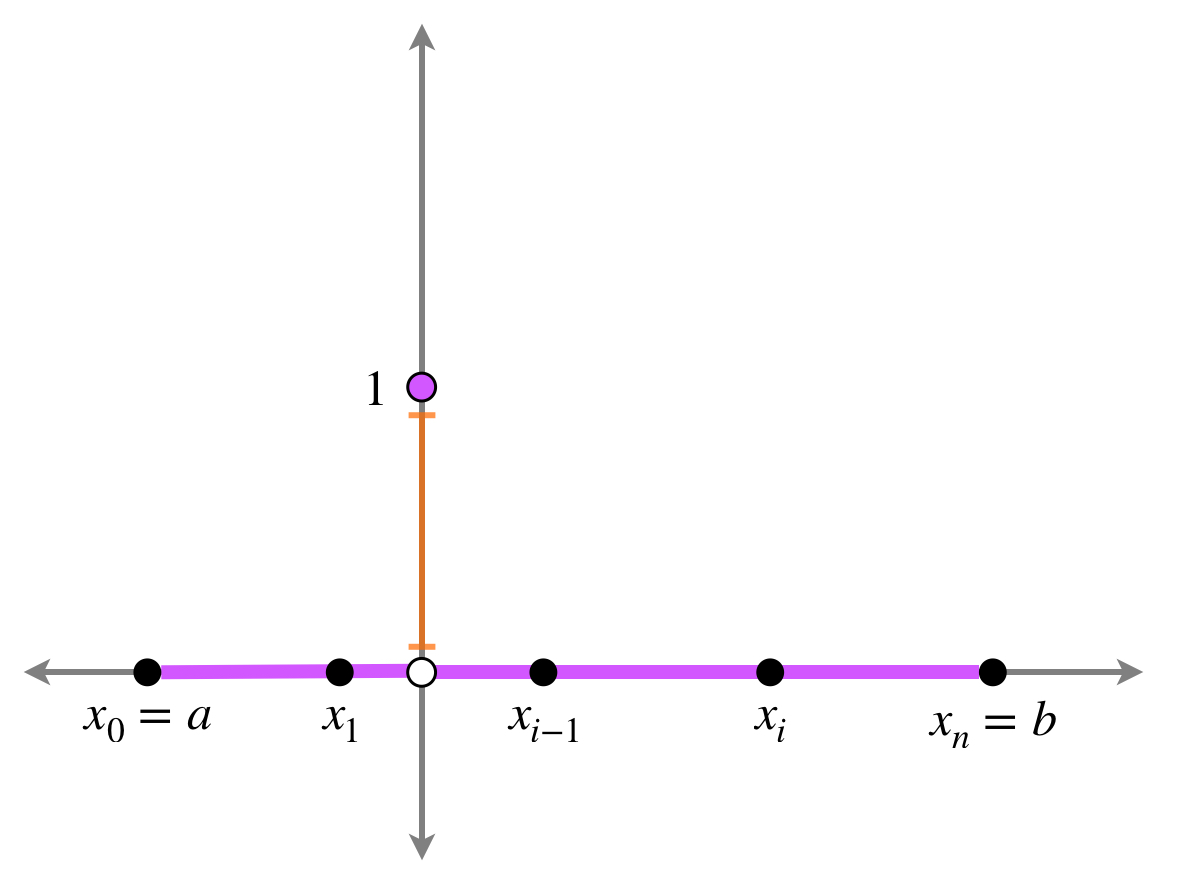
Sea $[a,b]$ un intervalo con el $\, 0$ en su interior y $f:[a,b] \to \mathbb{R}$ tal que \begin{equation*} f(x) = \begin{cases} 1 & \text{si $x = 0$} \\ 0 & \text{si $x \neq 0$} \end{cases} \end{equation*} Entonces $S_P = 2 \,$ o $\, S_P = 0,$ de modo que $V=2.$
$f$ no es continua en un punto.
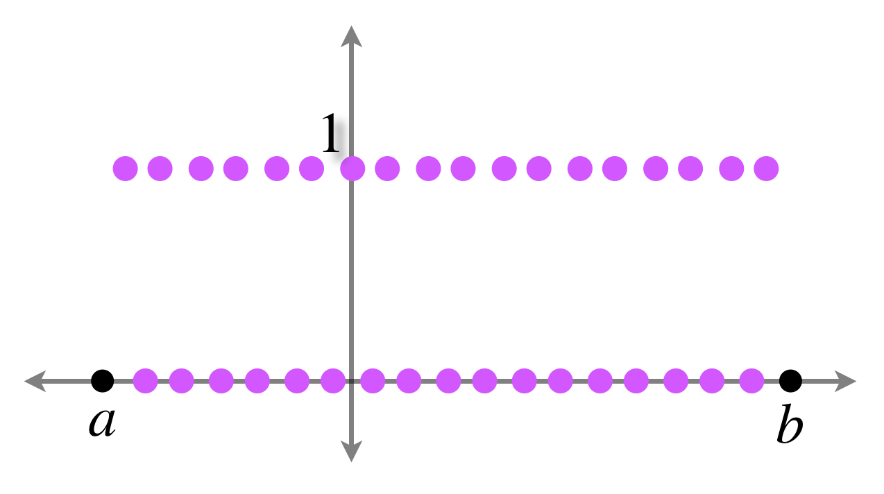
Sea $f:[a,b] \to \mathbb{R}$ la función de Dirichlet, es decir \begin{equation*} f(x) = \begin{cases} 1 & \text{si $x \, \in \, \mathbb{Q}$} \\ 0 & \text{si $x \, \notin \, \mathbb{Q}$} \end{cases} \end{equation*} Entonces $V = \infty.$
Gráfica de $f,$ la función de Dirichlet.
Las siguientes son propiedades de las funciones de variación acotada.
Proposición. Si $f$ es de variación acotada en $[a,b]$ entonces $f$ es acotada en $[a,b].$
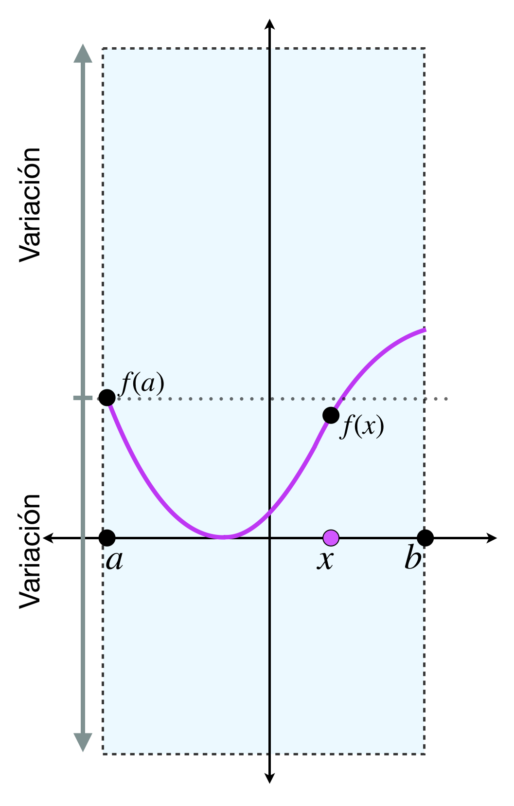
Demostración: Sea $x \in [a,b].$ Considera la partición $\{a, \, x, \, b\},$ entonces $$|f(x) \, – \, f(a)| \leq |f(x) \, – \, f(a)| +|f(b) \, – \, f(x)| \leq V.$$ Por lo tanto, $f$ es acotada en $[a,b].$
Para cualquier $x \in [a,b]$ se tiene que $f(x) \in [f(a)- V, f(a)+V].$
El regreso no es cierto, esto es, podemos tener una función acotada en $[a,b]$ pero que no sea de variación acotada. La función de Dirichlet ejemplifica esta situación. (Podrás ver otro caso también en la tarea moral de la siguiente entrada).
Proposición. Sean $f,g \,$ funciones de variación acotada en $[a,b]$ y sea $c \in \mathbb{R}.$ Entonces las funciones
$cf,$
$f+g \,$ y
$fg$
son de variación acotada en $[a,b].$ Además
$\dfrac{f}{g}$
también es de variación acotada en $[a,b]$ si existe $\varepsilon >0$ tal que $|g(x)| \geq \varepsilon$ para $x \in [a,b].$ La demostración queda como ejercicio.
Con las siguientes ideas tendremos recursos para aproximar mejor el valor de $V$ de una función.
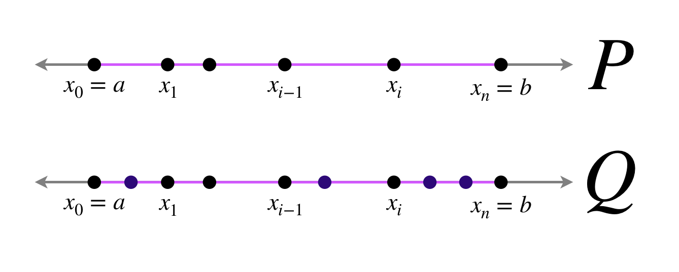
Definición. Refinamiento. Sean $P,Q \in \mathcal{P}_{[a,b]} \,$ tales que $P \subseteq Q,$ es decir, $Q$ tiene todos los puntos de $P$ y, posiblemente, algunos otros. Entonces decimos que $Q$ es un refinamiento de $P,$ o que $Q$ refina a $P.$
Representación de $Q$ como refinamiento de $P.$
Proposición. Si $Q$ es un refinamiento de $P,$ entonces $S_P \leq S_Q.$ La demostración la dejamos como ejercicio.
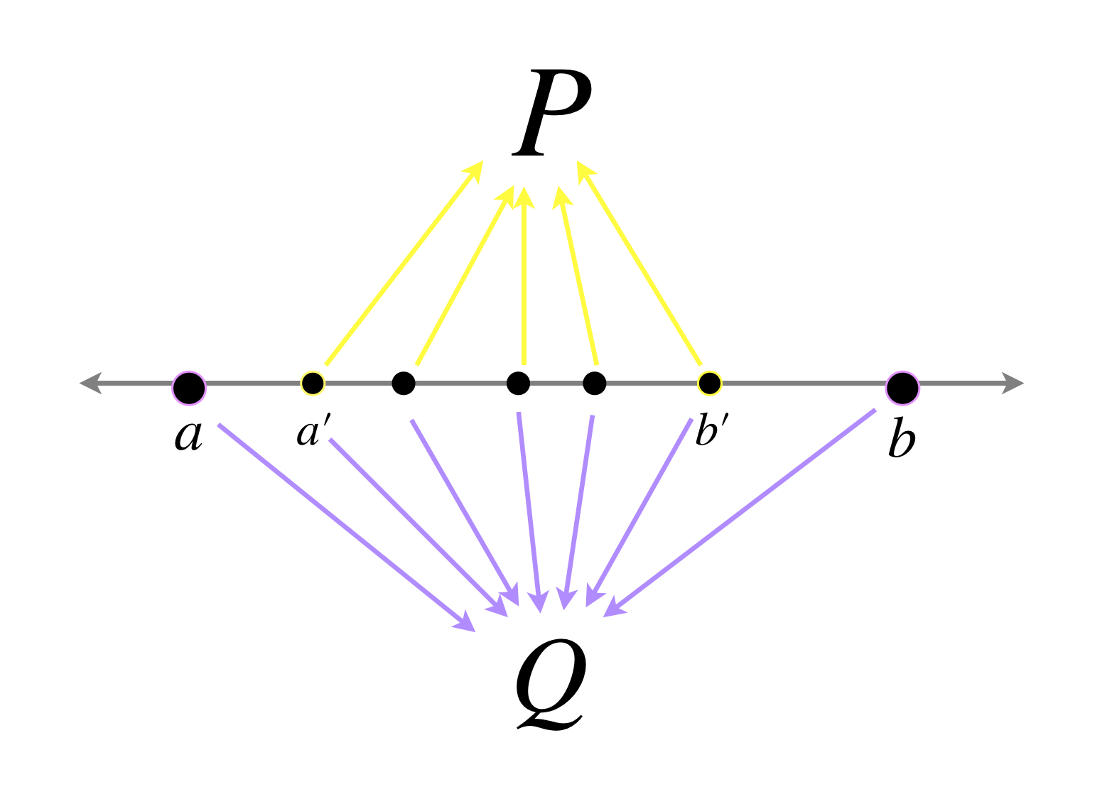
Proposición. Sea $f:[a,b] \to \mathbb{R}.$ Si $[a’,b’] \subseteq [a,b]$ entonces $V[a’,b’] \leq V[a,b],$ es decir, la variación potencialmente incrementa con el intervalo.
La partición $Q$ contiene a $P.$
Demostración: Sea $P= \{x_0= a’,…,x_n=b’\} \,$ una partición de $[a’,b’]$ y sea $Q = P \cup \{a,b\}.$ Claramente, $Q$ es partición de $[a,b]$ y \begin{align*} S_P[f;a’,b’] &= \sum_{i=1}^{n}|f(x_i) \, -\, f(x_{i-1})|\\ &\leq \sum_{i=1}^{n}|f(x_i) \, -\, f(x_{i-1})|+|f(x_0) \, -\, f(a)|+|f(b) \, -\, f(x_{n})|\\ &= S_Q[f;a,b] \end{align*}
lo cual indica que para cada $S_P, \, P \in \mathcal{P}_{[a’,b’]}$ existe $S_Q, \, Q \in \mathcal{P}_{[a,b]}$ tal que $S_P \leq S_Q.$ Por lo tanto $V[a’,b’] \leq V[a,b].$
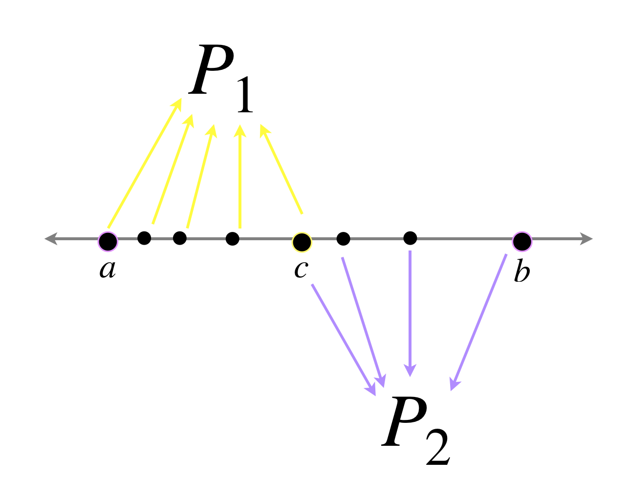
Proposición. Sea $f:[a,b] \to \mathbb{R}.$ Si $a < c < b$ entonces $$V[a,b] = V[a,c] + V[c,b].$$ Es decir, la variación es aditiva en intervalos adyacentes.
Demostración: Probemos primero que $V[a,c] + V[c,b] \leq V[a,b].$ Sea $P_1$ y $P_2$ particiones de $[a,c]$ y $[c,b],$ respectivamente. Entonces $P = P_1 \cup P_2$ es una partición de $[a,b].$
$P_1$ y $P_2$ generan una partición de $[a,b].$
En consecuencia $$S_{P_1}[f,a,c]+S_{P_2}[f,c,b] = S_P[f,a,b].$$ Ya que aún podrían existir otros valores más grandes de $S_{P’}[f,a,b]$ con $P’$ partición de $[a,b],$ se sigue que $V[a,c] + V[c,b] \leq V[a,b].$
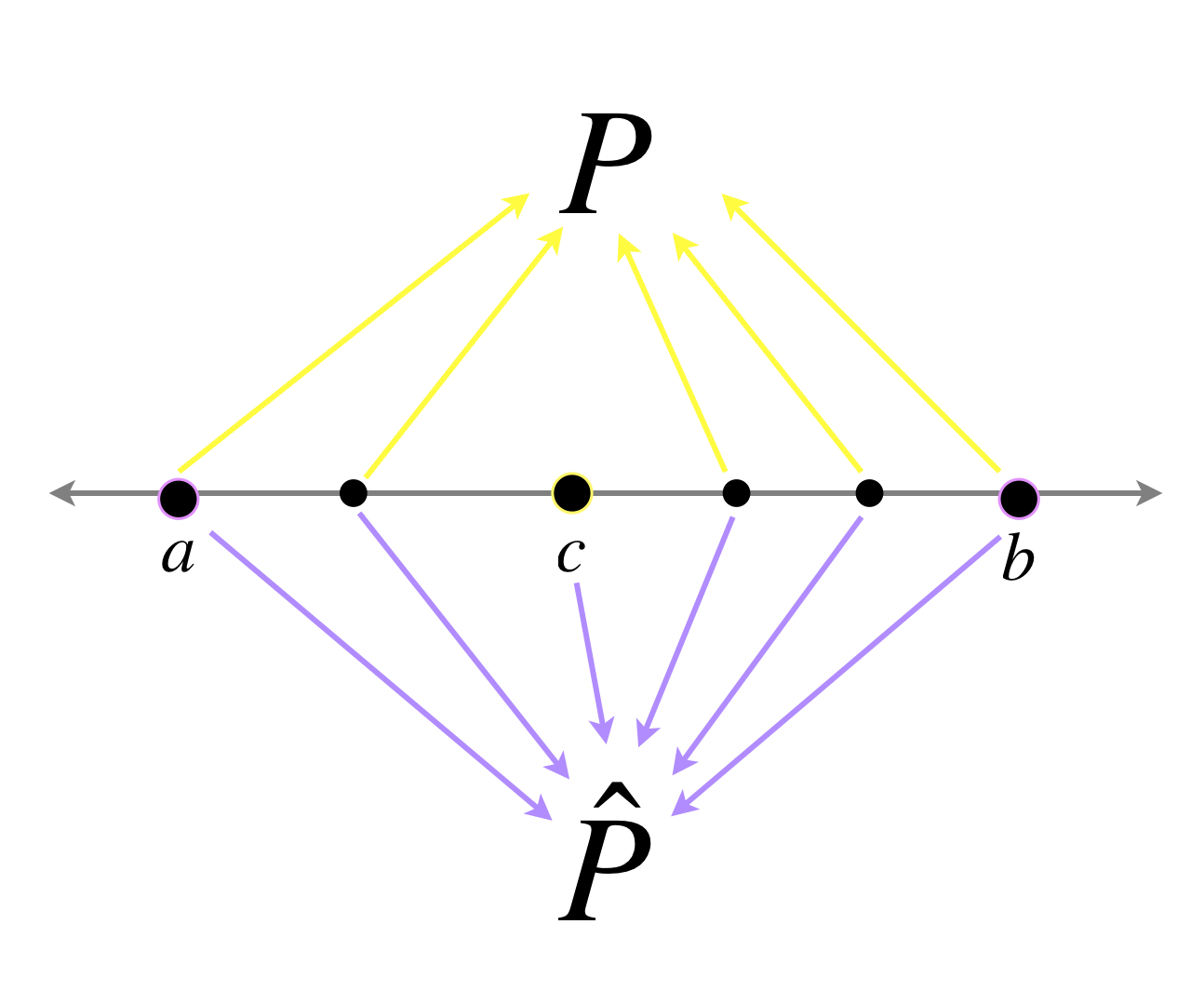
Ahora probemos que $V[a,b] \leq V[a,c] + V[c,b].$ Sea $P$ una partición de $[a,b]$ y $\hat{P}= P \cup \{c\}.$
$\hat{P}$ contiene a $P$ y a $\{c\}.$
Entonces $\hat{P}$ es un refinamiento de $P,$ y por la proposición que dejamos al lector tenemos $$S_P[f,a,b] \leq S_{\hat{P}}[f,a,b] = S_{P_1}[f,a,c]+S_{P_2}[f,c,b]$$ donde $P_1= \hat{P} \cap [a,c]$ y $P_2 = \hat{P} \cap [c,b].$ Por lo tanto $V[a,b] \leq V[a,c] + V[c,b],$ con lo que concluimos que
$$V[a,b] = V[a,c] + V[c,b].$$
Definición. Partes positiva y negativa de $x.$ Para cualquier $x \in \mathbb{R}$ definimos la parte positiva de $x$ como:
Nota que las partes positiva y negativa de un número real, satisfacen las siguientes relaciones:
$x^+,x^- \geq 0.$
$|x|=x^++x^- .$
$x = x^+-x^- .$
Definición. Suma de términos positivos y suma de términos negativos de $S_P.$ Sea $f:[a,b] \to \mathbb{R} \,$ y $P=\{x_0, \, x_1, \, … \, , x_{n-1}, \, x_n\}.$ Definimos la suma de términos positivos de $S_P$ como:
Demostración: Supongamos que $V$ es finito. Por (1) $$S_P^+ + S_P^- = S_P$$ y como $S_P \leq V,$ se sigue que \begin{align*} S_P^+ + S_P^- \leq V. \end{align*}
Ya que tanto $S_P^+$ como $S_P^- $ son no negativos, tenemos $$S_P^+ \leq V \, \Rightarrow \, S^+ \leq V.$$ De igual manera $$S_P^- \leq V \, \Rightarrow \, S^- \leq V.$$
Por lo tanto, si $V$ es finito, $S^+$ y $S^-$ también lo son.
Ahora supongamos que $S^+$ es finito. Despejando en (2), se cumple:
y por (8) \begin{align} S_{P_n} ^- \, \to \, S ^-, \end{align}
Por otro lado, por (1) $$S_{P_n}^+ + S_{P_n}^- = S_{P_n} \leq V$$ de modo que tomando el límite \begin{align} S^+ + S^- \leq V \end{align}
y de (7) y (15) concluimos finalmente
$$S^+ + S^- = V$$
que es (3).
Finalizamos esta sección con el siguiente
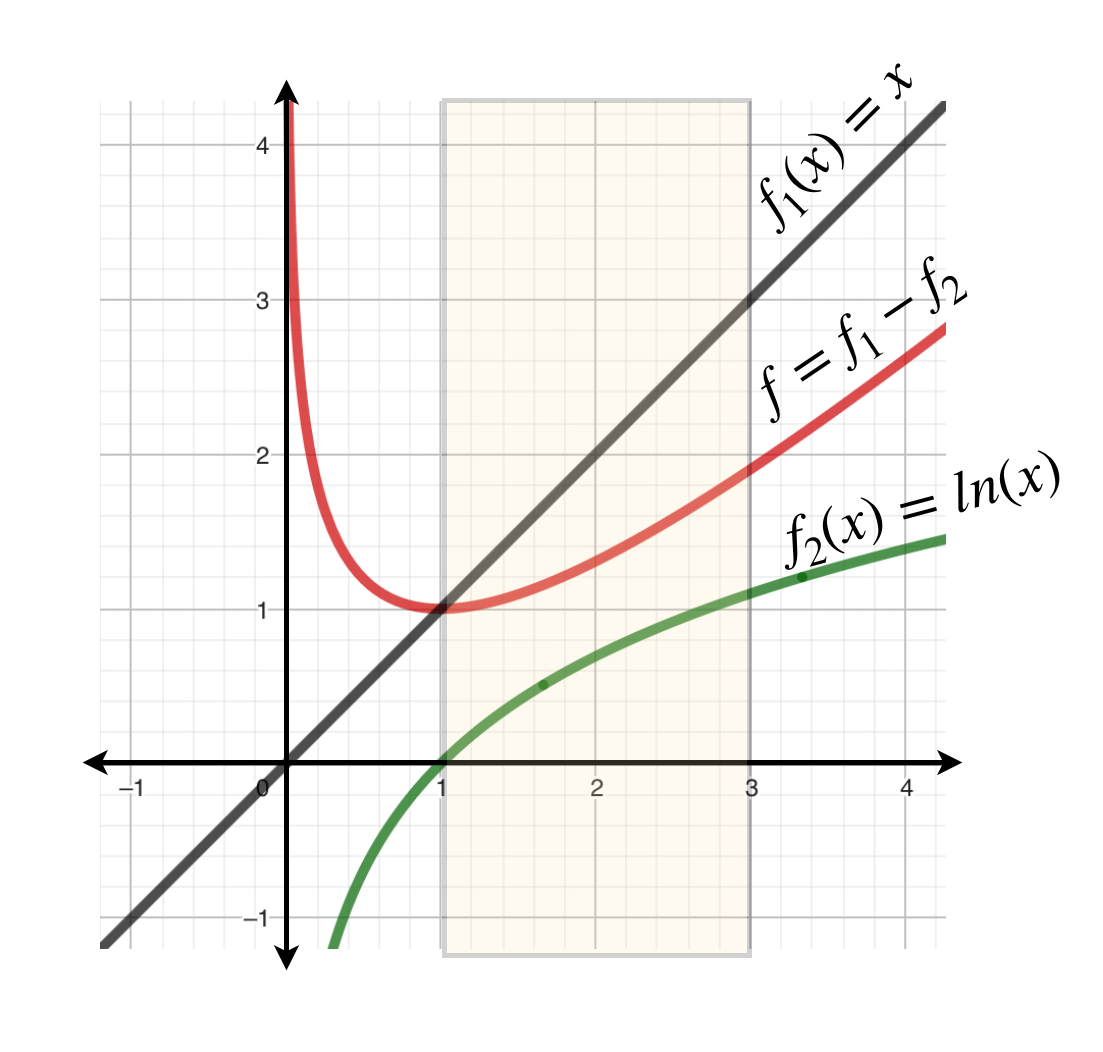
Corolario.Teorema de Jordan. Una función $f:[a,b] \to \mathbb{R}$ es de variación acotada en $[a,b]$ si y solo si puede ser expresada como la diferencia de dos funciones crecientes acotadas en $[a,b].$
La función en rojo es diferencia de las otras dos. Por lo tanto es de variación acotada en $[1,3].$
Demostración: Supón que $f$ es de variación acotada. Por un resultado visto arriba, sabemos que $f$ es de variación acotada en cada subintervalo $[a,x]$ con $x \in [a,b].$ Para cada $x,$ sean $S(x) ^+$ y $S(x) ^-$ las variaciones positiva y negativa de $f$ en $[a,x].$ Es sencillo demostrar que estas funciones son crecientes y acotadas en $[a,b],$ (ver tarea moral), y aplicando el teorema anterior en cada $[a,x],$ \begin{align*} && S(x) ^+ \, – \, S(x) ^- &= f(x) \, – \, f(a) \\ &\Rightarrow&f(x) &= (S(x) ^+ +f(a)) \, – \, S(x) ^- \end{align*}
Como $S(x)$ es creciente y acotada, también lo es $(S(x) ^+ +f(a))$, de modo que $f$ es la diferencia de dos funciones crecientes y acotadas.
En contraparte, supongamos que $f = f_1 \, – \, f_2,$ donde $f_1$ y $f_2$ son funciones crecientes y acotadas en $[a,b].$ De acuerdo con el primer ejemplo, ambas funciones son de variación acotada. Finalmente, por un resultado enunciado arriba, $ f_1 \, – \, f_2 = f \,$ es de variación acotada.
Más adelante…
Seguiremos con el estudio de las funciones de variación acotada y conectaremos con curvas rectificables, una concepción de cómo considerar la longitud de una curva que podría no coincidir, con medir la gráfica de la misma.
Tarea moral
Verifica la variación de cada función de los ejemplos enunciados arriba.
Demuestra que si $f,g \,$ son funciones de variación acotada en $[a,b]$ y $c \in \mathbb{R},$ entonces las funciones $$cf, \, f+g \, \, \text{ y } \, \, fg$$ son de variación acotada en $[a,b].$ Además $$\frac{f}{g}$$ también es de variación acotada en $[a,b]$ si existe $\varepsilon >0$ tal que $|g(x)| \geq \varepsilon$ para $x \in [a,b].$
Prueba que si $Q$ es un refinamiento de $P,$ entonces $S_P \leq S_Q.$
Para cada $x,$ sean $S(x) ^+$ y $S(x) ^-$ las variaciones positiva y negativa de $f$ en $[a,x].$ Demuestra que estas funciones son crecientes y acotadas en $[a,b].$
Prueba que si $f:[a,b] \to \mathbb{R}$ es Lipschitz continua, entonces es de variación acotada.
Bibliografía
Wheeden, R.L., Zygmund, A., Measure and Integral. An Introduccion to Real Analysis. (2da ed.). New York: Marcel Dekker, 2015. Págs: 17-22.
La curvatura de una curva $\alpha : [a,b] \subset \mathbb{R} \rightarrow \mathbb{R}^n$ en un punto $\alpha(t_0)$ es la curvatura de la circunferencia osculatriz (osculadora), «la que más se parece a la curva cerca del punto».
¿Cuál es la curvatura de una circunferencia?
De todas las circunferencias que pasan por el punto, ¿cuál es la que más se parece a la curva?
Definamos la curvatura de una circunferencia de radio $r$ como el número $\textcolor{RoyalBlue}{\mathcal{K} = \frac{1}{r}}$
Observación «física»:
Supongamos que tenemos una circunferencia parametrizada con rapidez constante 1.
$\alpha (s)$ nos da la posición.
${\alpha}’ (s)$ nos da la velocidad.
${\alpha}^{\prime \prime} (s)$ nos da la aceleración.
$\big\| {\alpha}’ (s) \big\| = 1$
$\big\| {\alpha}’ (s) \big\|^2 = 1$ constante.
Como la aceleración es perpendicular a la velocidad, se cumple que $ \big\langle {\alpha}’ (s) , {\alpha}^{\prime \prime} (s) \big\rangle = 0$
$ \big\langle {\alpha}’ (s) , {\alpha}’ (s) \big\rangle \equiv 1$ derivando $ \big\langle {\alpha}^{\prime \prime} (s) , {\alpha}’ (s) \big\rangle + \big\langle {\alpha}’ (s) , {\alpha}^{\prime \prime} (s) \big\rangle \equiv 0$
¿Cuál es la relación que hay entre $\mathcal{K}$ y ${\alpha}^{\prime \prime} (s)$ ?
Circunferencia de radio $1$ parametrizada con rapidez unitaria
$\alpha (t) = (\cos (t), \sin (t))$
${\alpha}’ (t) = ( – \sin (t) , \cos (t))$
$\big\| {\alpha}’ (t) \big\| = 1$
Circunferencia de radio $2$ parametrizada con rapidez unitaria
$\big\| {\alpha}^{\prime \prime} (s) \big\| = \frac{1}{r}$ es la «curvatura».
En general, dada una curva $\alpha : I \subset \mathbb{R} \rightarrow \mathbb{R}^n$ si ${\alpha \, }’ (t_0) \neq \vec{0}$, podemos definir «el» vector tangente unitario como $$\textcolor{ForestGreen}{\vec{T} (t_0) = \frac{{\alpha \, }’ (t_0) }{ \big\| {\alpha \, }’ (t_0) \big\|}}$$
Si la curva está parametrizada con rapidez unitaria $\alpha (s) $ tal que existe ${\alpha}’ (s)$ con $\big\|{\alpha \, }'(s) \big\| = 1$ para toda $s$, se tiene que $$T(s) = {\alpha \, }’ (s)$$
Dada una curva $\alpha (t)$, de clase $\mathcal{C}^1$, podemos reparametrizarla con rapidez unitaria.
Si ${\alpha \, }’ (t) \neq \vec{0} \; \; \forall \, t$; decimos que la curva es «regular».
Buscamos una función $t = h(s)$ tal que $\beta = \alpha \circ h$ y ${\beta \, }’ (s) = {\alpha \, }’ (h(s)) h’ (s)$ y que cumple que $\big\| {\beta \, }’ (s) \big\| = 1$ entonces $\big\|{\beta\, }’ (s) \big\| = \big\|{\alpha \, }’ (h(s)) \big\| h’ (s)$, con $h$ una función creciente.
Por lo que $$h’ (s) = \frac{1}{ \big\|{\alpha \, }’ (h(s)) \big\|}$$
Si además podemos que ${\alpha}^{\prime \prime} (s) \neq \vec{0}$ entonces, definimos «el» vector normal $N (s)$ como $$\textcolor{NavyBlue}{N (s) = \frac{{\alpha}^{\prime \prime} (s)}{\big\|{\alpha}^{\prime \prime} (s) \big\|}}$$
Dada una curva $\alpha (t)$, si ${\alpha \, }’ (t) \neq 0$ y existe ${\alpha}^{\prime \prime} (t)$ entonces $${\alpha}^{\prime \prime} (t) = \lambda {\alpha \, }’ (t) + \beta (t) $$
donde ${\alpha}^{\prime \prime} (t)$ es la aceleración,
${\alpha \, }’ (t)$ es la aceleración tangencial, y
$\beta (t)$ es la aceleración normal.
Es decir $${\alpha}^{\prime \prime} (t) = \lambda T (t) + N (t) $$
¿Cuál es la circunferencia osculatriz?
El radio está dado por $$\textcolor{BrickRed}{\frac{1}{\big\|{\alpha}^{\prime \prime} (s_0) \big\|}}$$
El centro de la circunferencia osculatriz es $$\alpha (s_0) + \frac{1}{\big\|{{\alpha \, }’ \, }’ (s_0) \big\|}.N(s_0) $$ $$\alpha (s_0) + \frac{1}{\|{\alpha}^{\prime \prime} (s_0) \big\|}. \frac{{\alpha}^{\prime \prime} (s_0)}{ \big\|{\alpha}^{\prime \prime} (s_0) \big\|}$$ $$ \textcolor{BrickRed}{\text{Centro} = \alpha (s_0) + \frac{{\alpha }^{\prime \prime} (s_0)}{{\big\|{\alpha}^{\prime \prime} (s_0)} \big\|^2}}$$
En conclusión, la curvatura mide el cambio en la dirección comparado con el cambio en la longitud de arco recorrida.
En la siguiente imagen puedes observar una animación de lo explicado en esta entrada.