En coordenadas rectangulares la longitud de arco de una curva parametrizada la calculamos con la integral $$\int\limits_{t_0}^{t_1} \Big\|{\alpha}’ (t) \Big\| dt$$
Si $\alpha (t) = \big( x (t), y (t) \big)$, y ${\alpha}’ (t) = \big( x’ (t) , y’ (t) \big)$, entonces $$\int\limits_{t_0}^{t_1} \sqrt{ \big( x’ (t)\big)^2 + \big(y’ (t) \big)^2 \, } dt $$
¿Qué integral habría que calcular si la curva está en otras coordenadas?
Por ejemplo: en coordenadas polares, es decir, si conocemos $ r (t)$ y $\theta (t)$
Entonces
$ x (t) = r (t) \cos \big( \theta (t) \big)$
$ y (t) = r (t) \sin \big( \theta (t) \big)$
Derivando
$ x’ (t) = r’ (t) \cos \big( \theta (t) \big) \, – \, r (t) {\theta}’ (t) \sin \big( \theta (t) \big)$
$ y’ (t) = r’ (t) \sin \big( \theta (t) \big) \, + \, r (t) {\theta}’ (t) \cos \big( \theta (t) \big)$
Luego
$\begin{align*} \big( x’ (t)\big)^2 + \big(y’ (t) \big)^2 &= \Big( r’ (t) \cos \big( \theta (t) \big) \, – \, r (t) {\theta}’ (t) \sin \big( \theta (t) \big) \Big)^2 + \Big( r’ (t) \sin \big( \theta (t) \big) \, + \, r (t) {\theta}’ (t) \cos \big( \theta (t) \big) \Big)^2 \\ &= \textcolor{Green}{ {r’}^2 {\cos}^2 \theta (t)} \, – \, \cancel{ \textcolor{Red}{2 r’ (t) r (t) {\theta}’ (t) \cos \theta (t) \sin \theta (t)}} + \textcolor{DarkBlue}{r^2 (t) {{\theta}’}^2 (t) {\sin}^2 \theta (t) } \\ & + \textcolor{Green}{ {r’}^2 {\cos}^2 \theta (t)} + \cancel{ \textcolor{Red}{2 r’ (t) r (t) {\theta}’ (t) \cos \theta (t) \sin \theta (t)}} + \textcolor{DarkBlue}{r^2 (t) {{\theta}’}^2 (t) {\sin}^2 \theta (t)} \\ &= \Big( r’ (t) \Big)^2 + r^2 (t) \Big( {\theta}’ (t) \Big)^2 \end{align*} $
Entonces $$\int\limits_{t_0}^{t_1} \sqrt{ \Big( r’ (t) \Big)^2 + r^2 (t) \Big( {\theta}’ (t) \Big)^2 \, } dt$$
${}$
La «notación diferencial»
$$ ds^2 = dx^2 + dy^2 \; \; \longrightarrow \; \; \Big(\dfrac{ds}{dt}\Big)^2 = \Big(\dfrac{dx}{dt}\Big)^2 + \Big(\dfrac{dy}{dt}\Big)^2$$
Entonces $$\int ds = \int \dfrac{ds}{dt} dt$$
En coordenadas polares
$ds^2 = dr^2 + r^2 d{\theta}^2 \longleftrightarrow \Big(\dfrac{ds}{dt}\Big)^2 = \Big(\dfrac{dr}{dt}\Big)^2 + r^2 \Big(\dfrac{d \theta}{dt}\Big)^2$
Queremos que $ T \, o \, \beta = \alpha$
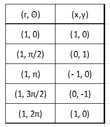
$T ( r, \theta) = (x, y)$
$x = r \cos \theta$
$y = r \sin \theta$
$x (t) = r (t) \cos \theta (t)$
$y (t) = r (t) \sin \theta (t)$
La «diferencial de T» ( o derivada de $T$)
$$DT = \begin{equation*} \left( \begin{matrix} \dfrac{\partial x}{\partial r} & \; \; & \dfrac{\partial x}{\partial \theta}\\ {} \\ \dfrac{\partial y}{\partial r} & \; \; & \dfrac{\partial y}{\partial \theta}\end{matrix} \right) \end{equation*}$$
Esta matriz es la transformación lineal que asocia vectores tangentes en el plano $r \theta$ con vectores tangentes en el plano $xy.$
Luego $DT \cdot {\beta}’ = {\alpha}’$
Entonces $ \begin{equation*} \left( \begin{matrix} \dfrac{\partial x}{\partial r} = \cos \theta & \; \; & \dfrac{\partial x}{\partial \theta} = – \, r \sin \theta \\ {} \\\dfrac{\partial y}{\partial r} = \sin \theta & \; \; & \dfrac{\partial y}{\partial \theta} = r \cos \theta \end{matrix} \right) \end{equation*}$
Entonces $$ \begin{equation*} \left( \begin{matrix} \cos \theta & \; \; & – \, r \sin \theta \\ {} \\ \sin \theta & \; \; & r \cos \theta \end{matrix} \right) \left( \begin{matrix} r’ \\ {} \\ {\theta}’ \end{matrix} \right) = \left( \begin{matrix} x’ \\ {} \\ y’ \end{matrix} \right) \end{equation*}$$
Luego
$ x’ = r’ \cos \theta \, – \, r {\theta}’ \sin \theta$
$ y’ = r’ \sin \theta \, + \, r {\theta}’ \cos \theta$
Para pedir la $\|{\alpha}’t\|$ usamos el producto punto
${\alpha}’ \cdot {\alpha}’=\|{\alpha}’\|^2$
$\sqrt{{\alpha}’ \cdot {\alpha}’}=\|{\alpha}’\|$
Si tenemos $T:V \longrightarrow W$ transf. lineal, y tenemos una función bilineal
$b:W \times W \longrightarrow \mathbb{R}$
podemos formar otra función bilineal B, tal que $B:V\times V \rightarrow \mathbb{R}$
$B( v_1 , v_2) := b(Tv_1, Tv_2)$
Vamos a medir el tamaño de los vectores en el plano $(r, \theta)$ no con la norma del producto punto sino con la norma de este producto escalar
$\begin{align*}B \Big( ({r’}_1, {\theta}’_1) , ({r’}_2, {\theta}’_2) \Big) &= b \Big( DT ({r’}_1, {\theta}’_1) , DT ({r’}_2, {\theta}’_2) \Big) \\ &= DT \begin{pmatrix} {r’}_1 \\ {\theta}’_1 \end{pmatrix} \cdot DT \begin{pmatrix} {r’}_2\\ {\theta}’_2 \end{pmatrix}\end{align*}$
$\begin{align*} \Big( {r’}_1 \cos \theta \, – \, r {\theta}’_1 \sin \theta , {r’}_1 \sin \theta \, + \, r {\theta}’_1 \cos \theta \Big) \cdot \Big( {r’}_2 \cos \theta \, – \, r {\theta}’_2 \sin \theta , {r}’_2 \sin \theta \, + \, r {\theta}’_2 \cos \theta \Big) \\ = \textcolor{Orange}{ {r}’_1 {r}’_2 {\cos}^2 \theta } \, – \, \cancel{ \textcolor{Red}{ {r’}_1 r {\theta}’_2 \cos \theta \sin \theta }} \, – \, \textcolor{DarkBlue}{{r}’_2 {\theta}’_1 \sin \theta \cos \theta } \\ + \textcolor{Green}{ {r}^2 {\theta}’_1 {\theta}’_2 {\sin}^2 \theta } + \textcolor{Orange}{ {r}’_1 {r}’_2 {\cos}^2 \theta } \, – \, \cancel{ \textcolor{Red}{ {r’}_1 r {\theta}’_2 \cos \theta \sin \theta }} \\ \, – \, \textcolor{DarkBlue}{{r}’_2 {\theta}’_1 \sin \theta \cos \theta } + \textcolor{Green}{ {r}^2 {\theta}’_1 {\theta}’_2 {\sin}^2 \theta } \\ = {r}’_1 {r}’_2 \, + \, {r’} {\theta}’_1 {\theta}’_2 \end{align*} $
Nueva norma para los vectores tangentes $\big( r’, {\theta}’ \big)$ en el plano $ ( r, \theta)$ $$\big\| \big( r’, {\theta}’ \big) \big\| : = \sqrt{{r’}^2 + r^2 {{\theta}’}^2 \, }$$
${}$
Jacobiano $= \begin{vmatrix} \cos \theta & \; \; \; & \; \; \sin \theta \\ \sin \theta & \; \; \; & \,- \ \cos \theta\end{vmatrix} = r \cos^2 \theta + r \sin^2 \theta = r $
En general, si tenemos un cambio de coordenadas
$ x = f (u, v)$
$ y = g (u, v)$
Sus derivadas son
$\dfrac{dx}{dt} = \dfrac{\partial x}{\partial u} \dfrac{du}{dt} + \dfrac{\partial x}{\partial v} \dfrac{dv}{dt}$
$\dfrac{dy}{dt} = \dfrac{\partial y}{\partial u} \dfrac{du}{dt} + \dfrac{\partial y}{\partial v} \dfrac{dv}{dt}$
Entonces
$\begin{pmatrix} \dfrac{dx}{dt} \\ {} \\ \dfrac{dy}{dt} \end{pmatrix} = \begin{pmatrix} \dfrac{\partial x}{\partial u} & \; \; & \dfrac{\partial x}{\partial v} \\{}\\ \dfrac{\partial y}{\partial u} & \; \; & \dfrac{\partial y}{\partial v} \end{pmatrix} \begin{pmatrix} \dfrac{du}{dt} \\ {} \\ \dfrac{dv}{dt} \end{pmatrix}$
Luego
$\begin{align*} \int\limits_{t_0}^{t_1} \big\|{\alpha}’ (t) \big\| dt &= \int\limits_{t_0}^{t_1} \sqrt{ \Big( \dfrac{dx}{dt}\Big)^2 \, + \, \Big( \dfrac{dy}{dt}\Big)^2 \, } dt \\ &= \int\limits_{t_0}^{t_1} H \Big( \dfrac{du}{dt} \, , \, \dfrac{dv}{dt} \Big) dt \end{align*} $
${}$
Longitud de arco de una curva en $\mathbb{R}^3$,
(*) en coordenadas cartesianas $$\textcolor{Red}{ds^2 = dx^2 \, + \, dy^2 \, + \, dz^2} $$
(*) en coordenadas cilíndricas $$\textcolor{Green}{ds^2 = dr^2 \, + \, r d{\theta}^2 \, + \, dz^2} $$
(*) en coordenadas esféricas $$\textcolor{DarkBlue}{ds^2 = dr^2 \, + \, r^2 \Big( d{\theta}^2 \, + \, {\sin}^2 \theta \; d{\varphi}^2 \Big) }$$