Ejemplo
Dada $f : \mathbb{R}^2 \rightarrow \mathbb{R}$ definida de la siguiente manera,
$$\begin{equation*} f (x, y) = \begin{cases} \dfrac{ \Big( \dfrac{x^2}{y}\Big)^2}{\Bigg( 1 + \Big( \dfrac{x^2}{y}\Big)^2 \Bigg)^4} & si & y \neq 0 \\ \\ 0 & si & y = 0 \end{cases} \end{equation*}$$
Consideremos primero $f_0 : \mathbb{R} \rightarrow \mathbb{R}$ donde $f_0 (x) = \dfrac{x^2}{\big( 1 + x^2 \big)^4}$ porque $f(x,y) = (f_0 \circ h) (x,y)$ con $h (x,y)=\dfrac{x^2}{y}$.
Nos preguntamos, ¿cómo es la gráfica de $f_0$? Para ello analizamos diferentes aspectos.
Podemos observar que:
(*) cuando $x \rightarrow \infty$ tenemos que $ f_0 (x) \rightarrow 0.$
(*) $f_0$ es par. Es decir, es simétrica respecto del eje $Y$.
(*) $f_0 (x) \geq 0$ para todo $x.$
(*) $f_0 (0) = 0.$
Entonces la gráfica de $f_0$ es

Cerca de cero $f_0 (x) \approx x^2$ y por tanto $f’_0 (0) = 0.$
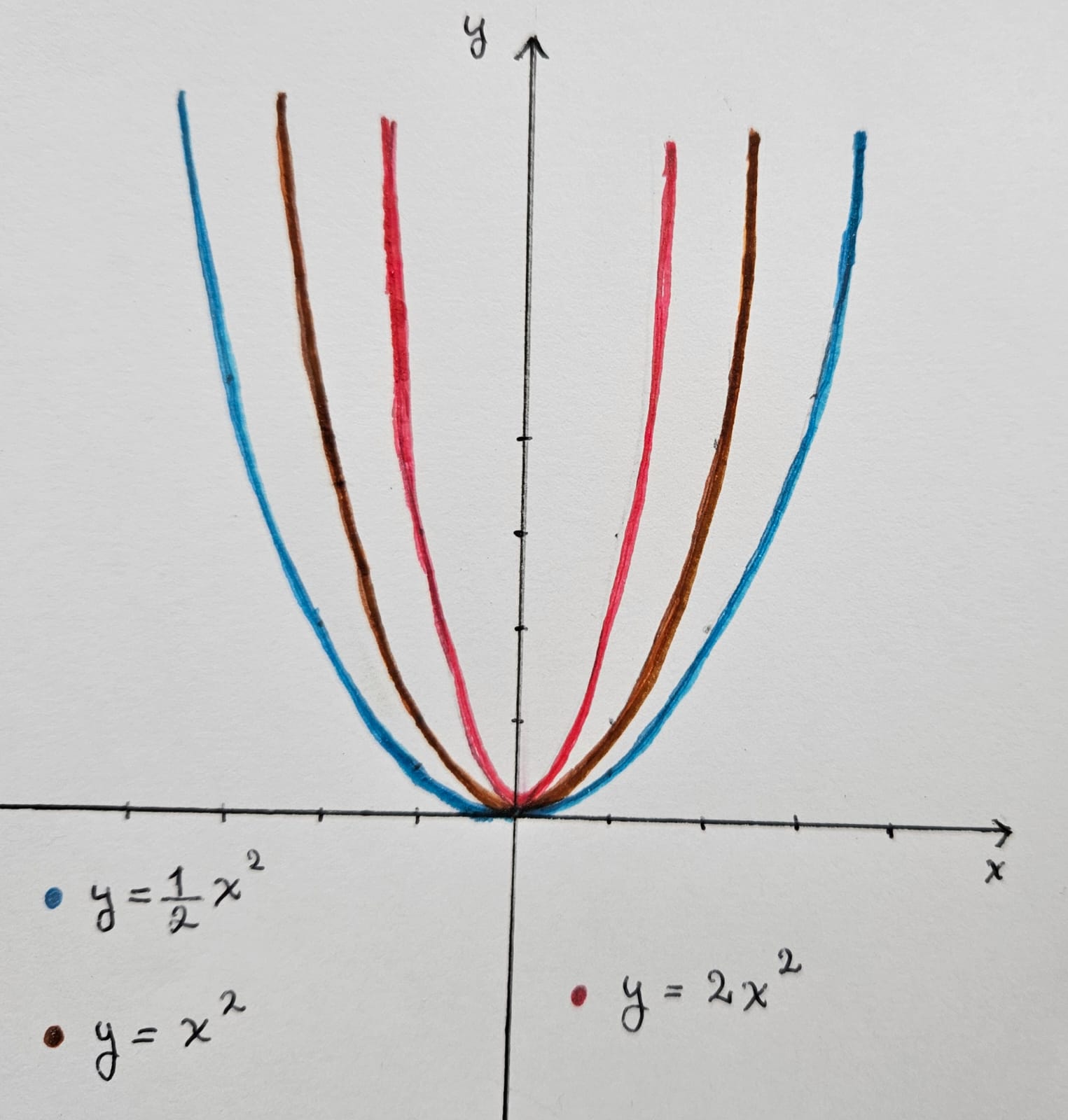
Consideremos $f_0 (\lambda x)$ con $\lambda > 0$ constante. ¿Cuál es el efecto en la gráfica?
Consideramos dos casos:
CASO 1: $ 0 < \lambda < 1$ por ejemplo $f_0 (\frac{x}{2})$
CASO 2: $ \lambda > 1$ por ejemplo $f_0 (2x)$
Recordemos una función análoga $ y = \sin x$
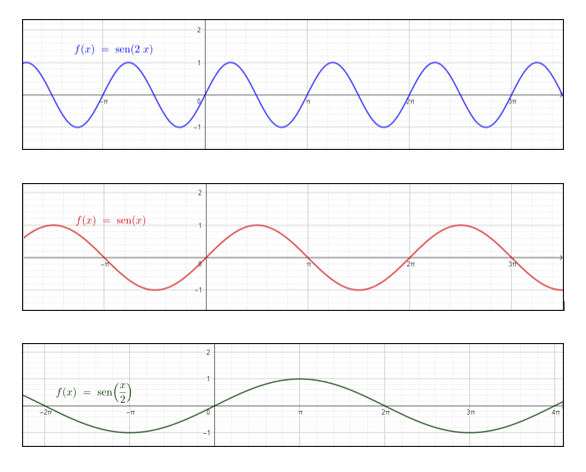
Observamos un $\lambda$ distinto para cada $y$.
Con $0 < \lambda < 1$ «alarga» la gráfica , y con $\lambda > 1$ la gráfica se «contrae».
Una primera idea sería $f_0 \Big( \dfrac{x}{y} \Big)$ cuando $ y \rightarrow 0$, ya que $\dfrac{1}{y} \rightarrow \infty $ la gráfica en el plano $XZ$ se contrae.
Sin embargo, a lo largo de rectas $ y = mx.$ $$f_0 \Big( \dfrac{x}{mx} \Big) = f_0 \Big( \frac{1}{m} \Big) \; \; \text{constante}$$
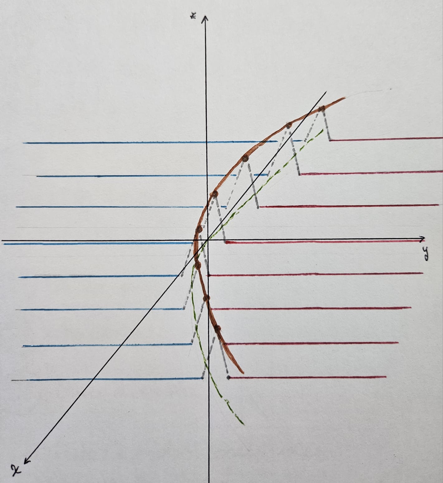
La función $f$ dada es «casi» constante a lo largo de parábolas $y = ax^2 \iff \dfrac{x^2}{y} = \dfrac{1}{a}$
Las curvas de nivel $f (x, y) = \mathcal{c}$ son parábolas perforadas, es decir $$ \Big\{ (x, y) \in \mathbb{R}^2 \Big| f (x, y) = \mathcal{c} \Big\}$$
donde $\mathcal{c} = \dfrac{\Big( \dfrac{x^2}{y} \Big)^2}{ \Bigg( 1 + \Big( \dfrac{x^2}{y} \Big)^2 \Bigg)^4}$
Para esto nos fijamos en la imagen inversa de $\mathcal{c}$ bajo $f_0$ tal que $$\Big\{ t \in \mathbb{R} \Big| f_0 (t) = \mathcal{c} \Big\} \Rightarrow \dfrac{t^2}{\Big( 1 + t^2 \Big)^4} = \mathcal{c}$$
En el siguiente enlace, puedes observar la gráfica de la función $f_0$ y su intersección con las rectas $z = c$ para $c \in [0, 0.11]$
https://www.geogebra.org/classic/arzvmgsv
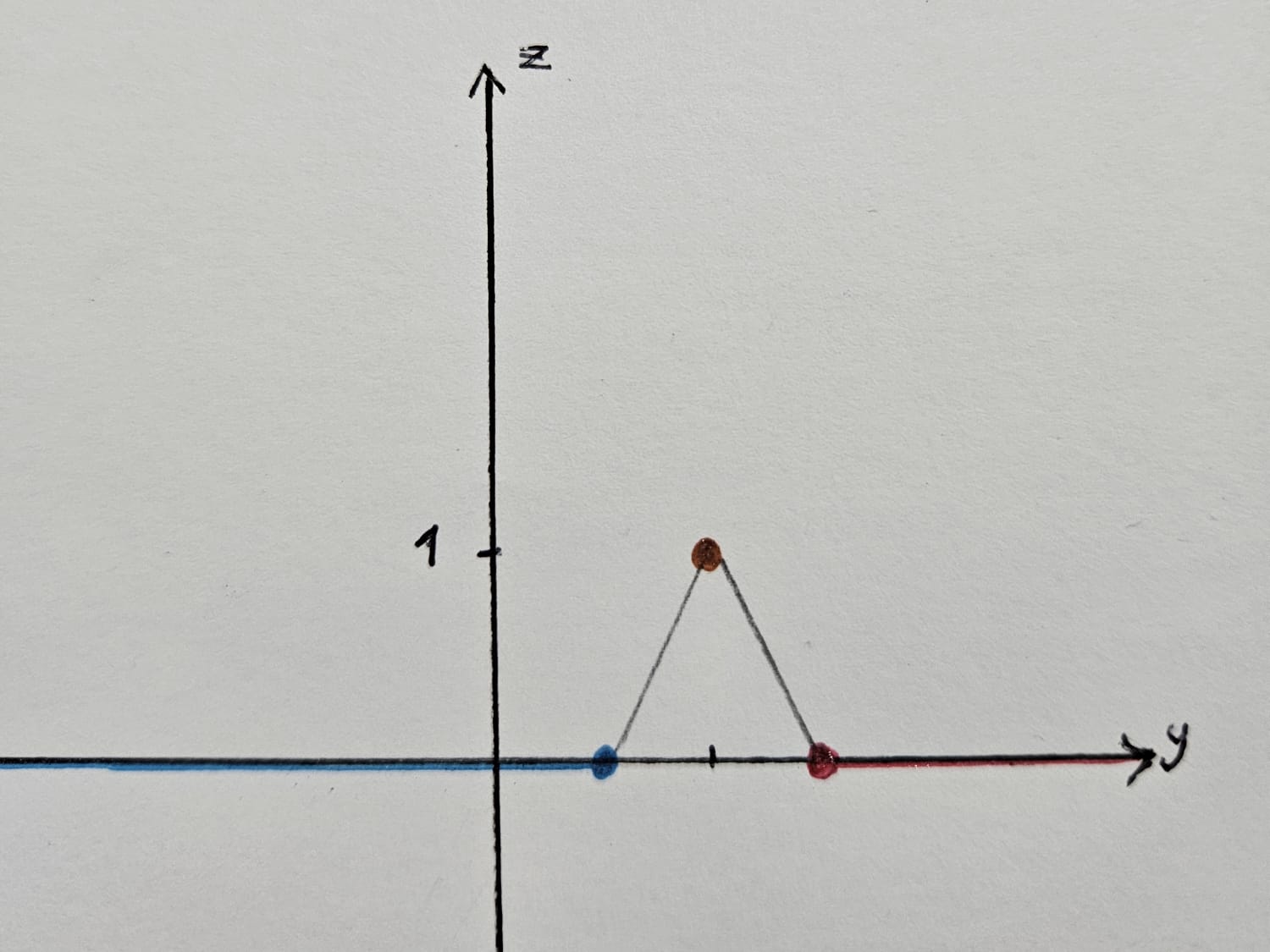
Si $\mathcal{c} > 0$ y $\mathcal{c}$ es menor que el máximo de $f_0$, entonces
$\Big\{ (x, y) \in \mathbb{R}^2 \big| f (x, y) = \mathcal{c} \Big\} = \Big\{ (x, y) \in \mathbb{R}^2 \big| f_0 \big( \frac{x^2}{y} \big) = \mathcal{c} \Big\}$ enotnces
$\Big\{ (x, y) \in \mathbb{R}^2 \big| \dfrac{x^2}{y} = t_1 \, ó \, \dfrac{x^2}{y} = t_2 \, ó \, \dfrac{x^2}{y} = t_3 \, ó \, \dfrac{x^2}{y} = t_4 \Big\} = \Big\{ (x, y) \in \mathbb{R}^2 \big| x^2 = t_1y \Big\} \setminus \Big\{ (0, 0) \Big\}$
Esto es la unión de cuatro parábolas menos el origen. En el siguiente enlace puedes observar una animación de lo que acabamos de analizar.
https://www.geogebra.org/classic/svzrgk7n
Además, si $\mathcal{c} = máx f_0$ el conjunto de nivel es la unión de dos parábolas menos el origen.
Si $\mathcal{c} < 0 $ entonces $f^{-1} (\mathcal{c}) = \emptyset.$
Si $\mathcal{c} > máx (f_0) $ entonces $f^{-1} (\mathcal{c}) = \emptyset.$
Si $\mathcal{c} = 0 $ entonces tenemos dos casos:
(*) $y = 0$
(**) $y \neq 0$ entonces $\dfrac{x^2}{y} = 0 $ y por tanto $ x = 0$, luego $f^{-1} (0) = $eje $X$ unión el eje $Y.$
${}$
Propiedades de este ejemplo:
(1) Todas las derivadas direccionales en el origen valen CERO.
(2) No es diferenciable en el origen.
(3) No es continua en el origen.
Analicemos cada propiedad:
(1) Las derivadas parciales
$\dfrac{\partial f}{\partial x} (0, 0) = 0$ y también $\dfrac{\partial f}{\partial y} (0, 0) = 0$
$\lim_{h \rightarrow 0} \dfrac{f (h, 0) \, – \, f (0, 0) }{h} = 0 $ y también $\lim_{k \rightarrow 0} \dfrac{f (0, k) \, – \, f (0, 0) }{k} = 0 $
Las otras derivadas direccionales $\vec{u} \in \mathbb{R}^2$, con $\big\| \vec{u} \big\| = 1$
Si $\vec{u} \neq \vec{e_1} , \vec{e_2}$ entonces la recta parametrizada $\alpha (t) = t \vec{u} $ pasa por el origen pero es distinta de los ejes.
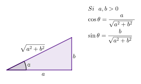
La derivada direccional $\lim_{t \rightarrow 0} \dfrac{f ( t \vec{u}) \, – \, f (\vec{0}) }{t}$ con $t \neq 0$ y con $\vec{u} = ( \cos \theta, \sin \theta)$
$t \vec{u} = ( t \cos \theta, t \sin \theta)$ donde $ x = t \cos \theta$ y $ y = t \sin \theta$
luego $ \dfrac{x^2}{y} = \dfrac{ t^2 \cos^2 \theta }{t \sin \theta} = t \cos \theta \cot \theta = t a $, donde $a$ es constante.
Entonces
$\begin{align*} f (x, y) = f_0 \Big( \dfrac{x^2}{y} \Big) &= \dfrac{ \Big( \dfrac{x^2}{y} \Big) }{\Bigg( 1 + \Big( \dfrac{x^2}{y} \Big)^2 \Bigg)^4} \\ &= \dfrac{ \big( t a \big) }{\big( 1 + \big( t a \big)^2 \big)^4} \\ &= \dfrac{t^2 a^2}{ \big( 1 + (t a)^2 \big)^4} \end{align*}$
Por lo que
$\begin{align*}\lim_{t \rightarrow 0} \dfrac{f ( t \vec{u}) \, – \, f (\vec{0}) }{t} &= \lim_{t \rightarrow 0} \dfrac{\dfrac{t^2 a^2}{\big( 1 + (t a)^2 \big)^4 \, – \, 0 }}{t} \\ &= \lim_{t \rightarrow 0} t \dfrac{a^2}{ (1+ (t a)^2)^4} \\ &= 0 \end{align*}$
(2) Para ver que no es diferenciable, primero veremos que no es continua.
(3) Para probar que $f$ no es continua basta dar una sucesión $\{ (x_n, y_n) \} \rightarrow (0, 0) $ tal que $ \{ f (x_n, y_n) \} \nrightarrow 0.$
Podemos acercarnos por una de las parábolas
$x_n = \dfrac{1}{n}, \; \; y_n = \dfrac{1}{n^2}$
Entonces $\dfrac{{x^2}_n}{y_n} = 1$ entonces $F (x_n , y_n) = f_0 (1) \neq 0$ y es constante.
Por lo tanto no es continua.
Y tampoco es diferenciable.
En el siguiente enlace puedes observar la gráfica de la función $f(x,y)$ que se analizó.