Sea $F : \mathcal{U} \subseteq \mathbb{R}^2 \rightarrow \mathbb{R}$ con derivadas parciales continuas $F_x$, $F_y$ en una vecindad de un punto $(x_0, y_0)$ tal que $F (x_0, y_0) = 0$ y además $F_y (x_0, y_0) \neq 0$, entonces existe un rectángulo $\big[ x_0 \, – \, \alpha , x_0 \, + \, \alpha \big] \times \big[ y_0 \, – \, \beta , y_0 \, + \, \beta \big]$ tal que para cada $x$ en el intervalo $\big[ x_0 \, – \, \alpha , x_0 \, + \, \alpha \big]$ la ecuación $F ( x, y) = 0$ tiene una solución $ y = f (x)$ con $ y_0 \, – \, \beta \leq y \leq y_0 \, + \, \beta. $
Dicha función $ f : \big[ x_0 \, – \, \alpha , x_0 \, + \, \alpha \big] \rightarrow \big[ y_0 \, – \, \beta , y_0 \, + \, \beta \big]$ satisface la condición $f (x_0) = y_0$ y para toda $ x \in \big[ x_0 \, – \, \alpha , x_0 \, + \, \alpha \big] $ cumple que
$F ( x, f (x) ) = 0$
$F_y ( x, f (x) ) \neq 0$
Más aún, $f$ es continua con derivada continua, y está dada por la ecuación
$$ f’ (x) = \, – \, \dfrac{F_x ( x, f (x) )}{F_y ( x, f (x) )}$$
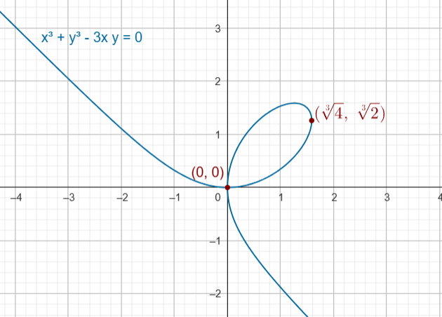
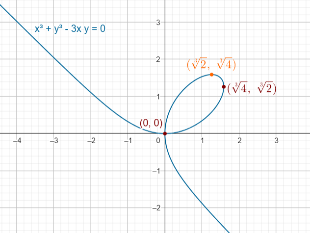
Si $y^3 = 0 \rightarrow y = 0$ por lo tanto $ y^2 = x \rightarrow x = 0$. Luego el punto es el $(0, 0)$
Si $ y^3 \, – \, 2 = 0 \rightarrow y = \sqrt[3]{2} $ por lo tanto $ y^2 = x \rightarrow (\sqrt[3]{2})^2 = x \rightarrow x = \sqrt[3]{4}$. Luego el punto es el $(\sqrt[3]{4}, \sqrt[3]{2})$
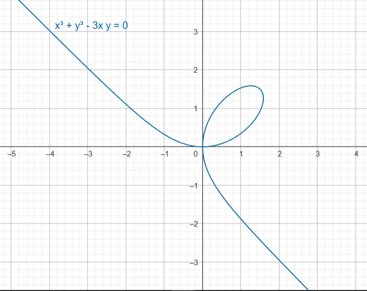
Podemos encontrar las coordenadas del punto en la hoja del primer cuadrante que está a una altura máxima.
Por lo que el gradiente de la función es $ \nabla F (0, 0) = \vec{0}$ en el punto $(0, 0) \in \mathcal{C}$, por lo que no es posible aplicar el teorema.
$ ( f \, \circ \, \alpha)’ (t) = 2 b^2 t \, – \, 12 a^2 b t^2 + 12 a^4 t^3 $ entonces $( f \, \circ \, \alpha)’ (0) = 0$
${( f \, \circ \, \alpha)}^{\prime \prime} (t) = 2 b^2 \, – \, 24 a^2 b t + 36 a^4 t^2 $ entonces ${( f \, \circ \, \alpha)}^{\prime \prime} (0) = 2 b^2 > 0 $. Si $ b \neq 0$. Entonces $ f \, o \, \alpha $ alcanza un mínimo relativo en 0.
Si $ b = 0 $ , $a = 1$ $ f ( \alpha ( t)) = 3 t^4$ que también tiene mínimo en $(0, 0)$.
De aquí concluimos que si restringimos el movimiento de las variables independientes a lo largo de rectas que pasan por el origen, entonces $f$ alcanza un valor mínimo.
(***) Ahora vamos a ver que $f$ no alcanza un mínimo local en el origen.
Para ello usaremos la negación de la definición de que $ f $ alcanza mínimo local en el punto $(x_0 , y_0)$.
Es decir queremos negar que:
existe una bola de radio $\delta$ con centro en el punto $(x_0 , y_0)$ en la cual todos los puntos $(x,y)$ cumplen que $f(x,y) \geq f(x_0 , y_0)$.
Es decir que para toda bola $B_{\delta} (x_0, y_0) $ existe algún punto $(x,y)$ en esa vecindad tal que $f (x, y) < f (x_0 , y_0)$
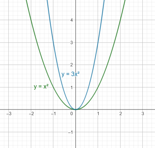
Sea $\delta > 0$, consideremos la parábola $ 2x^2$, tomemos un punto en esta parábola dentro de $B_{\delta} (0, 0) $ distinto del $(0, 0) $. En este punto $f (x, y) < 0 = f (0, 0)$, entonces $ f $ no alcanza un valor mínimo local en $(0, 0)$.
La matriz simétrica que define la parte de segundo grado de este polinomio $p(x,y)$ recibe el nombre de Matriz Hessiana de $f$ en el punto $(x_0, y_0)$.
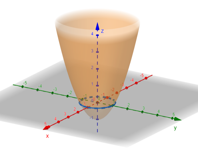
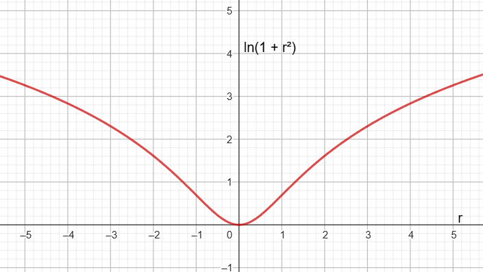
La gráfica de $f$ es $ \big\{ (x, y, z) \in \mathbb{R}^3 \Big| z = \ln (1 + x^2 + y^2) \big\} $ , una superficie de revolución girando la curva $ z = \ln (1 + x^2) $ alrededor del eje $z$.
$ \vec{w} $ es el vector velocidad usando $\beta$ como parametrización.
Los dos vectores velocidad $ \vec{v}$ y $\vec{w} $ son colineales. Además, si
$ h’ (0) > 0 $ tienen el mismo sentido, y si
$h’ (0) < 0 $ tienen sentidos contrarios.
${}$
Supongamos que $ \gamma (t) = \big( x (t), y (t) \big)$ es una curva parametrizada, y que $ x (t)$ , $y (t) $ son de clase $\mathcal{C}^2$.
Además
$\gamma’ (0) \neq \vec{0}$
${\gamma}^{\prime \prime} (0) \neq \vec{0}$
Se dice que la circunferencia osculatriz a una curva en un punto $P$ es la circunferencia que más se parece a la curva cerca del punto.
¿Cómo saber cuál es la circunferencia osculatriz en el punto $P$?
Si $\gamma $ estuviera parametrizada por longitud de arco, entonces el centro de la circunferencia osculatriz es $$ \gamma (0) + \dfrac{1}{\mathcal{K} (0)} \vec{n} (0)$$
donde $\vec{n} (0) $ es el vector normal unitario.
Y el radio de la circunferencia osculatriz es $\dfrac{1}{\mathcal{K} (0)}$
Sabiendo la curvatura y el vector normal tenemos toda la información necesaria. (no necesariamente tiene que ser en el punto CERO, puede ser un punto $t_0$ con $\gamma’ (t_0) $ y ${\gamma}^{\prime \prime} (t_0)$ distintas de CERO)
(*) Tenemos una fórmula para calcular $\mathcal{K} (t_0)$
(*) a. En el plano, basta conocer el vector tangente unitario $T (t_0) = \dfrac{ \gamma’ (t_0)}{ \big\| \gamma’ (t_0) \big\|}$. Solo hay dos opciones para $(u, v)$ puede ser $ (- \, v, u ) $ o también $ (v, \, – \, u) $